This is a Plain English Papers summary of a research paper called AI Denoises CT Scans: Clearer Images with Less Radiation?. If you like these kinds of analysis, you should join AImodels.fyi or follow us on Twitter.
The Critical Challenge of Noise in Low-Dose CT Imaging
Low-dose computed tomography (CT) reduces radiation exposure but increases image noise, potentially compromising diagnostic accuracy. This noise can obscure subtle structures and low-contrast lesions, leading to diagnostic errors. Traditional denoising approaches face significant limitations. Supervised methods require paired datasets (clean and noisy images) that are ethically and practically difficult to obtain in medical settings. Self-supervised approaches often need multiple noisy images of the same scene and rely on deep networks like U-Net that offer little insight into the denoising mechanism.
Filter2Noise (F2N) addresses these challenges through an interpretable framework, adaptive filtering, and single-image training. Unlike Zero-Shot Noise2Noise and other self-supervised methods, F2N combines superior performance with transparency and user control—critical features for clinical applications.

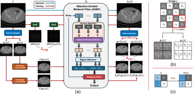
Figure 1: (a) The Filter2Noise (F2N) denoising pipeline. (b) The downsampling strategy, following ZS-N2N. (c) Our proposed Euclidean Local Shuffle (ELS).
The Filter2Noise Framework: Methodology with Interpretability at its Core
Self-supervised single-image denoising methods typically construct noisy image pairs from a single noisy image via downsampling. While effective, most network-based approaches operate as "black boxes," offering limited insight into the denoising process. The Filter2Noise framework integrates Attention-Guided Bilateral Filtering (AGBF) as its core denoising mechanism to provide an interpretable alternative.
How Attention-Guided Bilateral Filtering Makes Denoising Transparent
Standard bilateral filters use fixed global parameters, limiting their adaptability to spatially varying noise. AGBF fundamentally changes this by making filter parameters spatially dependent and conditioned on input image content. This allows the filter to adaptively adjust its smoothing behavior based on local image features and noise levels.
The AGBF architecture employs a dual-attention module to estimate spatially varying parameters (σᵣ, σₓ, σᵧ) for each image patch at every denoising stage. In contrast to conventional bilateral filters that apply uniform smoothing across the image, AGBF dynamically adjusts to local image characteristics. This approach shares conceptual similarities with Two-Stage Deep Denoising approaches but focuses on transparency and parameter efficiency.
The standard bilateral filter computes a denoised pixel as a weighted average of neighboring pixels, using fixed spatial and range standard deviations. AGBF extends this by making these parameters adaptive and content-dependent, significantly improving denoising performance while maintaining interpretability.
Providing Radiologists with Control Over the Denoising Process
A key advantage of AGBF is its inherent interpretability. As the denoising process is controlled by learned, spatially varying standard deviations, visualizing these parameters offers insight into the denoising behavior. Higher σᵣ values indicate stronger smoothing in areas with greater noise intensity.
Moreover, AGBF allows users to adjust the standard deviation maps post-training, enabling region-specific denoising. For example, radiologists can increase σᵣ for suspected lesions, enhancing diagnostic confidence and transparency. Users can also define upper limits for filter parameters to prevent excessive blurring, with these limits tailored to anatomical regions to accommodate different noise properties or preferences.
Training a Denoiser Without Clean Reference Images
The F2N framework leverages multi-stage AGBF and exploits image self-similarity across scales to address spatially correlated noise. The training strategy incorporates a multi-scale reconstruction loss, edge preservation regularization, and the proposed Euclidean Local Shuffle (ELS).
Creating Training Pairs from a Single Image
Following Zero-Shot Noise2Noise (ZS-N2N), two downsampled images are generated from the noisy input using 2×2 convolution with specific kernels. These kernels average different pixel combinations, creating two distinct noisy views of the same content that can be used for self-supervised training.
Breaking Correlated Noise with Euclidean Local Shuffle
To address spatially correlated noise in low-dose CT, F2N introduces the Euclidean Local Shuffle technique. While downsampling alone struggles to decorrelate noise, ELS disrupts local patterns by rearranging pixels in 2×2 blocks based on minimum Euclidean distance.
For a 2×2 block with pixel values (a,b,c,d), ELS calculates the Euclidean distances between all pixel pairs, identifies the minimum distance, and swaps those pixels. This operation disrupts noise correlation while preserving local image statistics, preventing the model from learning a trivial identity mapping. This innovation relates to concepts explored in Positive2Negative, which also addresses challenges in self-supervised denoising.
Self-Supervised Loss Function Design
For training, F2N uses a total loss combining reconstruction and regularization components. The reconstruction loss works across multiple scales to ensure effective denoising, while the edge preservation regularization prevents over-smoothing of important structural details. This balanced approach ensures high-quality denoising without sacrificing critical diagnostic information.
Performance Evaluation: Filter2Noise in Action
The experimental evaluation assessed F2N against other self-supervised single-image methods, focusing on denoising performance, parametric efficiency, interpretability, and key design impacts.
Testing Across Different CT Reconstruction Kernels
The evaluation utilized the Mayo-2016 and Mayo-2020 low-dose CT datasets from the NIH AAPM-Mayo Clinic Grand Challenge. The experiments considered the crucial impact of reconstruction kernels on noise characteristics—smoother kernels like B30 produce correlated noise, while sharper kernels like D45 generate more random noise.
The Mayo-2016 dataset was divided into B30 and D45 subsets (526 slices each), while the Mayo-2020 dataset (641 slices) provided additional noise profiles. All 512×512 pixel images were denoised using self-supervised single-image methods without requiring training data.
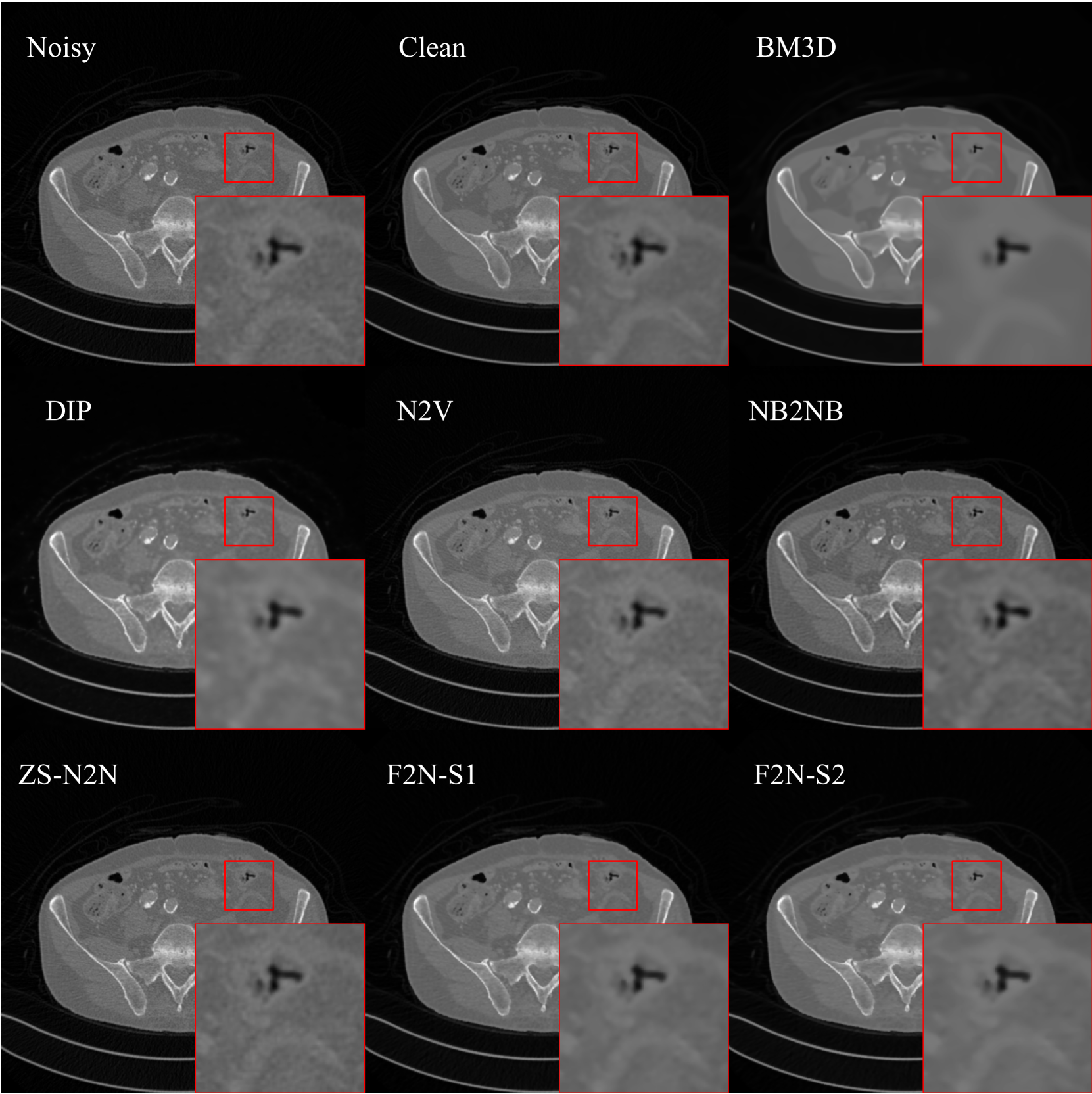
Figure 2: Denoising comparison across the Mayo-2016 B30 dataset.
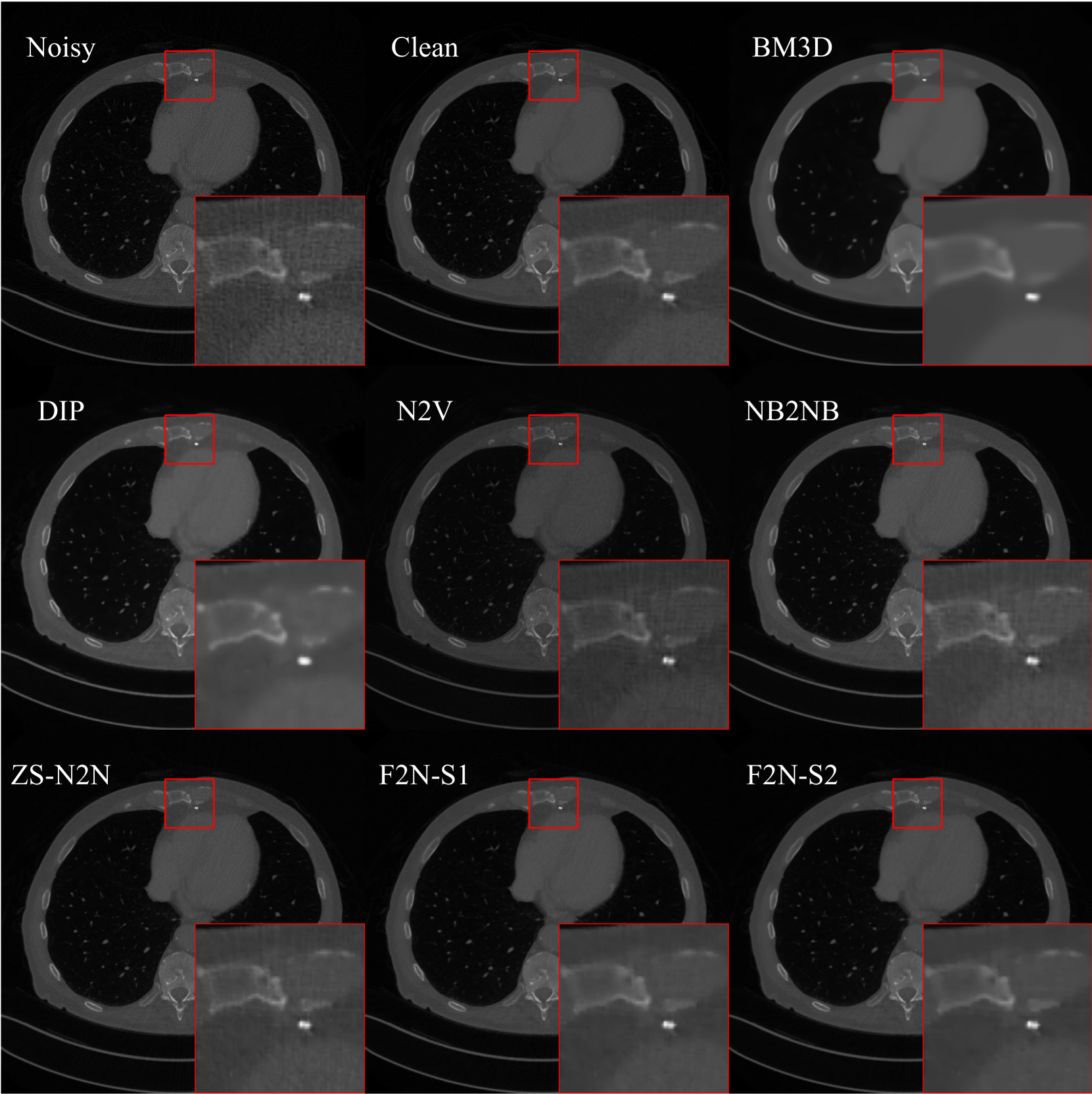
Figure 3: Denoising comparison across the Mayo-2016 D45 dataset.
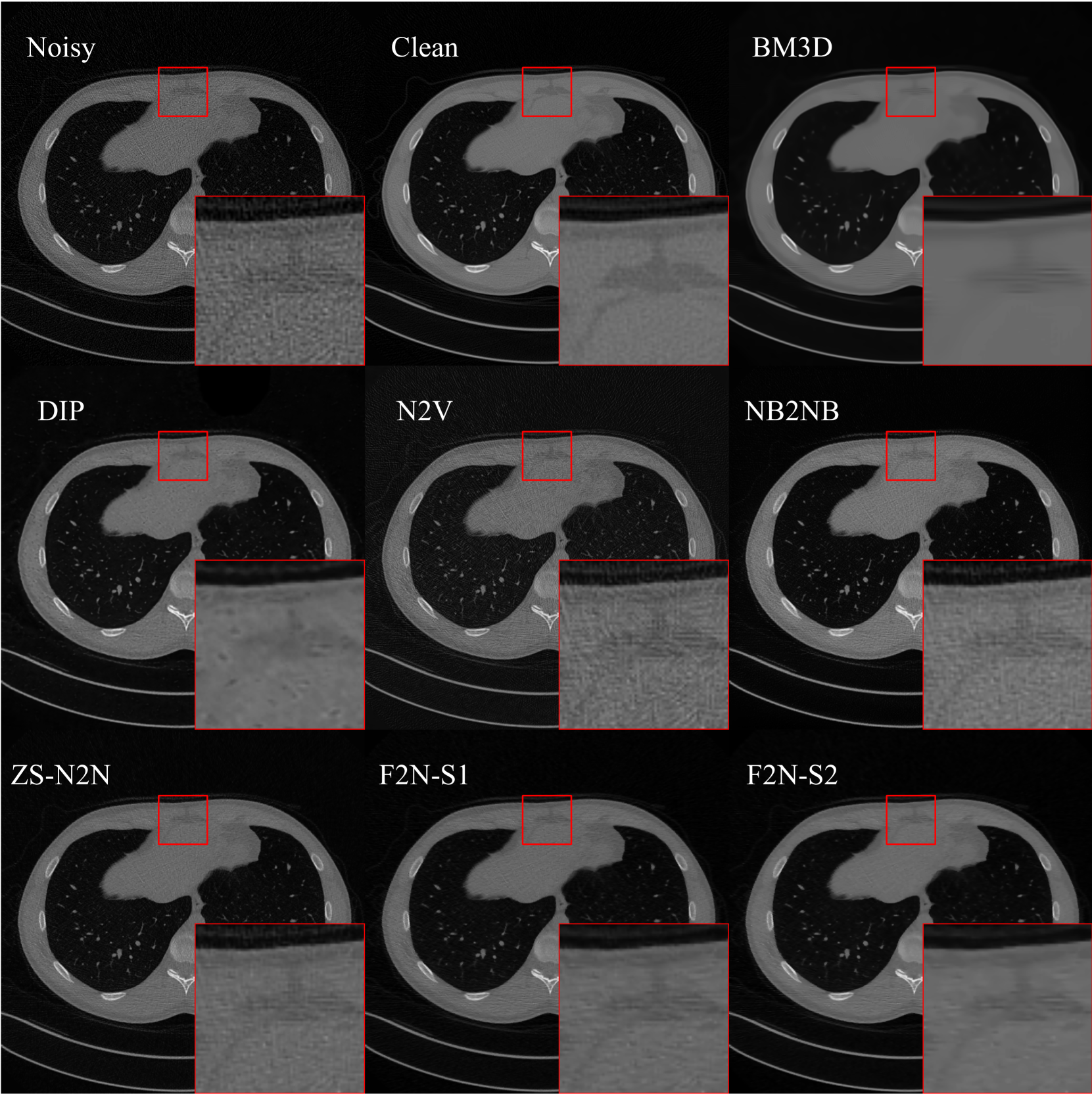
Figure 4: Denoising comparison across the Mayo-2020 dataset.
Filter2Noise Outperforms Existing Methods with Fewer Parameters
The evaluation compared F2N to established methods including BM3D, Deep Image Prior (DIP), Noise2Void (N2V), Neighbor2Neighbor (NB2NB), and Zero-Shot Noise2Noise (ZS-N2N).
| Method | Mayo-2016 B30 | Mayo-2016 D45 | Mayo-2020 | GPU Time | # Params. | |||
|---|---|---|---|---|---|---|---|---|
| PSNR (dB) | SSIM | PSNR (dB) | SSIM | PSNR (dB) | SSIM | |||
| BM3D (TIP2007) [3] | 37.15 | 89.41 | 35.48 | 87.80 | 36.50 | 88.27 | 3 sec. | – |
| DIP (CVPR2018) [23] | 37.94 | 90.74 | 36.23 | 84.97 | 36.69 | 85.92 | 3 min. | 2.2 M |
| N2V (CVPR2019) [9] | 33.63 | 88.45 | 35.78 | 86.73 | 33.56 | 83.68 | 10 min. | 2.2 M |
| NB2NB (TIP2022) [6] | 36.63 | 89.79 | 37.70 | 89.89† | 36.97 | 86.09 | 90 sec. | 1.3 M |
| ZS-N2N (CVPR2023) [13] | 35.13 | 84.33 | 38.01† | 89.24† | 37.21† | 88.43 | 22 sec. | 22 k |
| F2N-S1 w/o ELS (Ours) | 35.11 | 84.24 | 37.05 | 87.33 | 36.98 | 86.92 | 10 sec. | 1.8 k |
| F2N-S2 w/o ELS (Ours) | 35.62 | 85.08 | 37.14 | 87.41 | 36.44 | 86.97 | 20 sec. | 3.6 k |
| F2N-S1 (Ours) | 39.54 | 91.35 | 37.79 | 89.17 | 37.19 | 89.92 | 11 sec. | 1.8 k |
| F2N-S2 (Ours) | 39.72 | 91.78 | 38.03 | 89.61 | 37.28 | 90.09 | 20 sec. | 3.6 k |
Table 1: Results on the Mayo Low-Dose CT Challenge. B30/D45: reconstruction kernels. F2N-S1/S2: one/two AGBF layers. Inference time per slice is measured on an NVIDIA RTX 4070 Super GPU. Two-sided paired t-tests compare each method with F2N-S2. † indicates no significant difference (p>0.05).
While BM3D effectively reduces noise, it tends to over-smooth fine details. ZS-N2N and NB2NB perform well on Mayo-2016 D45 and Mayo-2020 but struggle with the correlated noise in Mayo-2016 B30. Filter2Noise consistently achieves superior performance, with the two-stage version (F2N-S2) achieving the highest PSNR and SSIM values in most cases.
Notably, F2N-S2 achieves these results while using only 3.6k parameters—significantly fewer than other methods. This demonstrates the effectiveness of AGBF and the training strategy. Even the single-stage F2N-S1 performs strongly, indicating that a single AGBF layer can denoise effectively.
The approach taken by F2N offers advantages over other self-supervised medical image denoising techniques like Neighboring Slice Noise2Noise, particularly in scenarios where only a single slice is available. The implementation and code for Filter2Noise are available on GitHub, enabling further research and clinical applications.
Looking Inside the Denoising Process
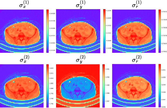
Figure 5: Visualization of the spatially varying standard deviation maps from F2N-S2.
The visualization of spatially varying standard deviation parameters provides insight into the denoising behavior of F2N-S2. The larger σᵣ⁽¹⁾ compared to σᵣ⁽²⁾ indicates that the first stage performs the primary noise reduction, with the second stage refining the result. The consistently larger σₓ compared to σᵧ suggests preferential smoothing along the x-direction. The spatial variation within each map demonstrates the adaptive nature of the filtering, reflecting local image content and noise characteristics.
Understanding Key Design Choices Through Ablation
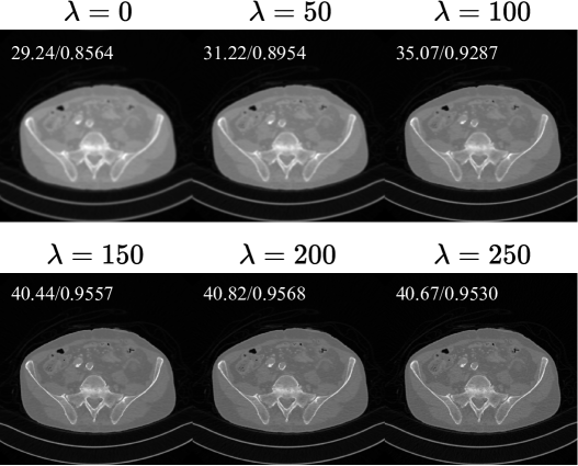
Figure 6: Ablation study on λ (Equation 10). PSNR and SSIM values are shown.
The ablation study focused on the regularization weight λ and the presence of ELS, as performance was most sensitive to these factors. λ controls the trade-off between noise reduction and edge preservation. Lower values lead to blurring (weaker edge preservation), while higher values result in sharper images but with more residual noise. This illustrates the importance of proper parameter tuning.
The Euclidean Local Shuffle also proved critical—without it, performance degrades significantly, especially with spatially correlated noise (as seen in the B30 dataset). This confirms the importance of addressing noise correlation in low-dose CT denoising.
Advancing Medical Image Denoising with Interpretable AI
Filter2Noise represents a significant advancement in medical image denoising, offering a rare combination of high performance, interpretability, user control, and parameter efficiency. On the Mayo Clinic 2016 low-dose CT dataset, F2N outperforms the leading self-supervised single-image method (ZS-N2N) by 4.59 dB PSNR while using fewer parameters.
The interpretable nature of F2N addresses a crucial need in medical imaging, where understanding the denoising process can be as important as the result itself. The ability to visualize and adjust filter parameters post-training provides radiologists with unprecedented control over the denoising process, allowing them to tailor it to specific diagnostic tasks or regions of interest.
Future work will focus on accelerating inference through custom CUDA kernel implementation and extending F2N to other medical imaging modalities. These improvements will further enhance the clinical utility of this promising approach, providing medical professionals with a powerful, transparent tool for improving image quality in low-dose CT and potentially other imaging modalities.