Introduction Computer Vision
Computer vision refers to a set of processes and techniques that allow a computer to have the ability to understand elements of the real world from digital images.
Preprocessing Images
According to Gonzalez and Woods (2018), there is no consensus among authors on where image processing ends and computer vision begins.
The terms refer to groups of necessary computational processes that require operations at different levels.
Low level:
Image preprocessing: Operation that will consist of cleaning unnecessary data within the image, validating dimensions and corrupted images, restructuring colors and other operations if necessary.
Medium Level:
Segmentation: Search for real-world objects, detecting shapes such as lines and curves
Classification: This is a technique that searches for characteristics within images to categorize each one with its due label.
High Level:
Essential step for inferring final results. Seeking to evaluate the classified objects.
Application Areas
Optical Character Recognition
As the name suggests, the game's functionality is to detect characters. It is widely used for images, PDFs, and others. For example, it can capture words and sentences in different types of files.
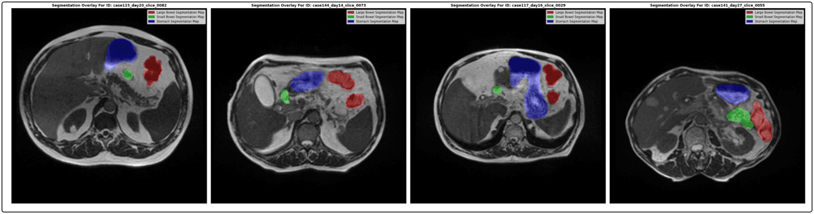
Medical image analysis
Used to detect tumors, organs, blood vessels and other possibilities
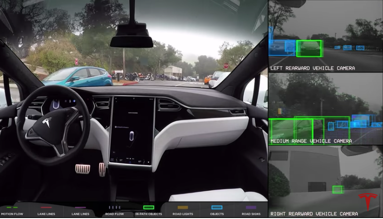
Autonomous vehicles
Vehicles that have the ability to detect objects in the real world, making decisions without the need for humans.
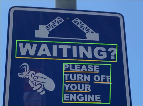
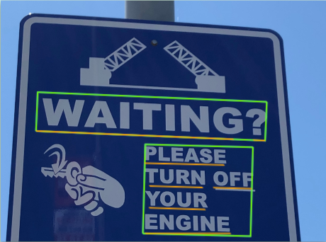
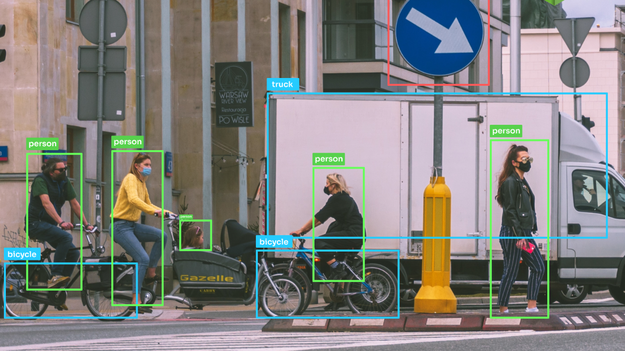
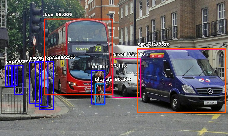
Object detection
Detect objects such as cars, people, signs, buildings and more.
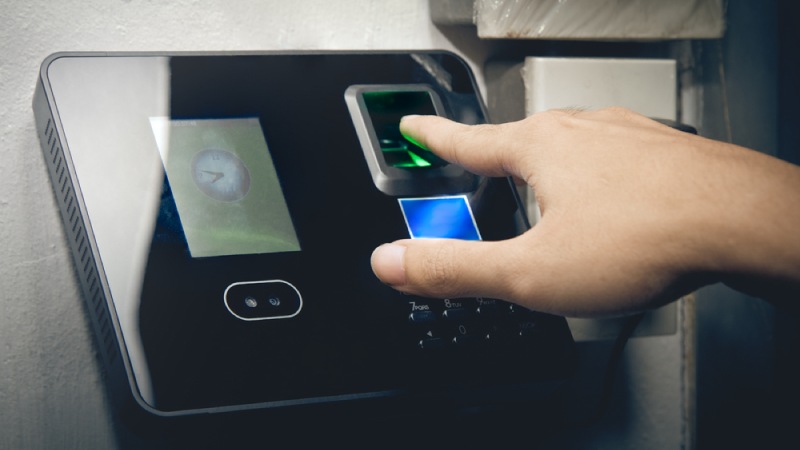
Biometrics
Detect individual characteristics of each user to be used as identifiers.
Tracking
Track specific objects within an image.
Fundamentals of Digital Imaging
Workflow for Computer Vision Systems
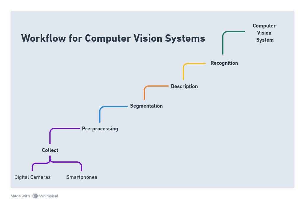
Image collection
Most of the images found in the world are digital, these images are captured by sensors, sensors that have an energy input from a light source. This lighting includes visible light, x-rays, radars, infrared and ultrasound. Thus, the sensor output has a continuous voltage characteristic. In this way, it is possible to digitize the captured data to generate a response, in this case an image.
There are two situations within this:
Sampling: Obtaining a discrete and finite set of samples of the continuous data provided by the sensor in the form of a two-dimensional MxN matrix, defining a number of pixels in the matrix.
Quantization: Obtaining a discrete and finite set of intensity levels such as brightness for each pixel sample obtained from the continuous data provided by the sensor.
Digital Image
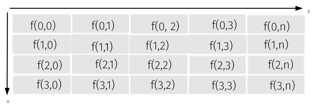
A digital image is a set of finite integers of pixels, with each pixel having an integer value that represents the level of intensity (brightness) of the pixel.
A digital image is defined with a function f(x, y):
- x and y are integers that represent the spatial coordinates,
- f is an integer that represents the level of intensity or brightness at each coordinate x, y
The digital image is represented by a matrix with M rows and N columns, where:
- Visual Intensity
- Numerical Intensity
- The individual elements of each matrix are called pixels
import requests
from PIL import Image
import matplotlib.pyplot as plt
import numpy as npdata = requests.get('https://images.pexels.com/photos/31096175/pexels-photo-31096175/free-photo-of-black-and-white-aerial-view-of-busy-city-intersection.jpeg?auto=compress&cs=tinysrgb&w=1260&h=750&dpr=1').content
f = open('1.jpg','wb')
f.write(data)
f.close()data = requests.get('https://images.pexels.com/photos/19996987/pexels-photo-19996987/free-photo-of-brasil-game-show-2019.jpeg?auto=compress&cs=tinysrgb&w=1260&h=750&dpr=1').content
f = open('2.jpg','wb')
f.write(data)
f.close()data = requests.get('https://images.pexels.com/photos/15128096/pexels-photo-15128096/free-photo-of-red-bus-parked-beside-a-sidewalk.jpeg?auto=compress&cs=tinysrgb&w=1260&h=750&dpr=1').content
f = open('3.jpg','wb')
f.write(data)
f.close()Original Image
image = Image.open('/kaggle/working/1.jpg')
image_array = np.array(image)
plt.figure(figsize=(6, 6))
plt.imshow(image_array)
plt.axis("off")
plt.show()
Pixels with visual intensities
tile = image_array[0:25, 0:25, :]

print(f'Tile shape: {tile.shape}')

plt.figure(figsize=(6, 6))
plt.imshow(tile)
plt.axis("off")
plt.show()Tile shape: (25, 25, 3)
Pixels with numerical intensities
fig, ax = plt.subplots(1, 4, figsize=(30, 7))

for i, channel in enumerate(['Red', 'Green', 'Blue', 'Grayscale']):
    if i < 3:
        ax[i].imshow(tile[:, :, i], cmap='gray')
        ax[i].set_title(f'{channel} Channel')
    else:
        grayscale = np.dot(tile[..., :3], [0.2989, 0.5870, 0.1140])
        ax[i].imshow(grayscale, cmap='gray')
        ax[i].set_title(f'{channel} Channel')

for i in range(25):
    for j in range(25):
        for k in range(3):
            ax[k].text(j, i, tile[i, j, k], ha='center', va='center', color='white', fontsize=6)
        ax[3].text(j, i, np.round(grayscale[i, j], 2), ha='center', va='center', color='white', fontsize=6)

for a in ax:
    a.axis('off')

plt.show()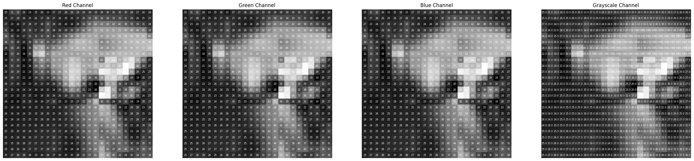
Original Image
image = Image.open('/kaggle/working/2.jpg')
image_array = np.array(image)
plt.figure(figsize=(30, 7))
plt.imshow(image_array)
plt.axis("off")
plt.show()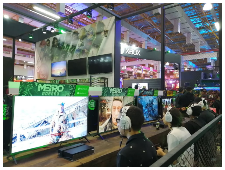
Pixels with visual intensities
tile = image_array[0:25, 0:25, :]

print(f'Tile shape: {tile.shape}')

plt.figure(figsize=(6, 6))
plt.imshow(tile)
plt.axis("off")
plt.show()Tile shape: (25, 25, 3)
Pixels with numerical intensities
fig, ax = plt.subplots(1, 4, figsize=(30, 7))

for i, channel in enumerate(['Red', 'Green', 'Blue', 'Grayscale']):
    if i < 3:
        ax[i].imshow(tile[:, :, i], cmap=f'{channel}s')
        ax[i].set_title(f'{channel} Channel')
    else:
        grayscale = np.dot(tile[..., :3], [0.2989, 0.5870, 0.1140])
        ax[i].imshow(grayscale, cmap='gray')
        ax[i].set_title(f'{channel} Channel')

for i in range(25):
    for j in range(25):
        for k in range(3):
            ax[k].text(j, i, tile[i, j, k], ha='center', va='center', color='white', fontsize=6)
        ax[3].text(j, i, np.round(grayscale[i, j], 2), ha='center', va='center', color='white', fontsize=6)

for a in ax:
    a.axis('off')

plt.show()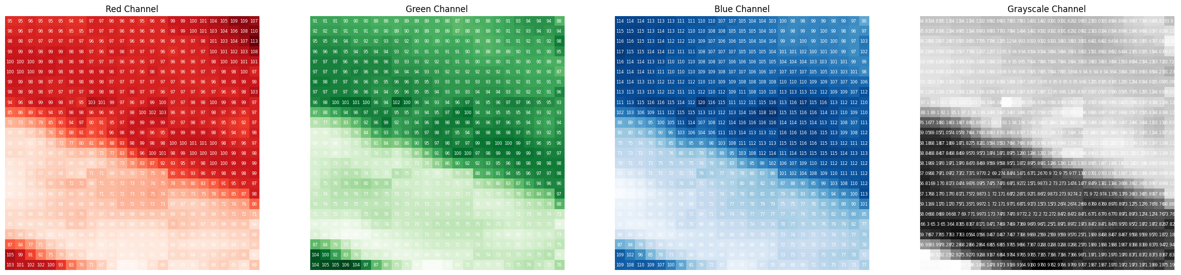
The number of intensity levels L of a digital image is a power of 2.
where:
- ( L ) is the total number of possible intensity levels in the image.
- ( k ) is the number of bits used to represent each intensity level.
Intensity Range
Intensity levels are integers in the range ([0, L-1]).
This range is known as the intensity scale. It determines the minimum and maximum values that a pixel can assume in an image.
For example:
- For ( L = 256 ) (( k = 8 ) bits), the intensity values range from ( 0 ) to ( 255 ).
- In this case:
- The value ( 0 ) represents the lowest intensity, associated with black.
- The value ( 255 ) represents the highest intensity, associated with white. - All intermediate values correspond to different shades of gray.
Relationship Between Bits and Image Quality
The number of bits per pixel (( k )) is directly related to the quality and richness of detail in an image:
The higher the value of ( k ), the greater the number of intensity levels ( L ).
This allows the image to represent tonal variations more accurately, improving the visual perception of subtle details.
For example:
- 1 bit per pixel (( k = 1 )):
- Only 2 intensity levels (( L = 2 )), representing black and white (binary image).
- 8 bits per pixel (( k = 8 )):
- 256 intensity levels (( L = 256 )), allowing richer gray tones.
- 16 bits per pixel (( k = 16 )):
- 65,536 intensity levels (( L = 65,536 )), used in high-definition or scientific images.
Neighborhood
The neighborhood of a pixel refers to the adjacent pixels (neighbors) of a central pixel in a given region of the image. This definition is fundamental for several operations in digital image processing.
Neighborhood Applications
The analysis of the neighborhood of a pixel is widely used in:
- Spatial Filtering: For smoothing (removing noise) and enhancing images.
- Image Segmentation: To divide the image into regions of interest based on characteristics such as color, texture or intensity.
- Edge Detection: To locate edges and contours that define shapes and objects in an image.
Neighborhood Types
The number of pixels considered as neighbors is determined based on the area around the central pixel. The most common types include:
- Neighborhood-4:
- Includes the pixels directly above, below, to the left and to the right of the central pixel.
- Total of 4 neighbors.
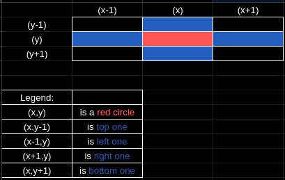
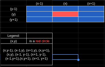
- Neighborhood-8:
- Includes the pixels of neighborhood-4 plus the pixels located diagonally in relation to the central pixel.
- Total of 8 neighbors.
Introduction to Color in Computer Vision
Color as a Descriptor
Color is a useful descriptor for identifying and extracting features from objects in an image. Human vision perceives colors through combinations of primary colors of light, which are fundamental for visual representation in computational models.
Linear Color Spectrum
The linear color spectrum of visible light can be divided into six broad regions: violet, blue, green, yellow, orange, and red. Each region represents a range of distinct wavelengths within the visible spectrum.

Source: Wikimedia Commons
Primary Colors of Light
Primary colors of light are fundamental for the creation of other colors. These include:
- R - Red
- G - Green
- B - Blue
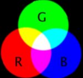
Additive Model
The primary colors of light can be added together to produce secondary colors:
- C - Cyan
- M - Magenta
- Y - Yellow
Mixing all three primary colors of light or a secondary with its opposite primary color at the correct intensities results in the production of white light.
Color Models
The two main color models or color spaces used in computer vision are:
RGB - Red, Green, Blue
In the RGB model, images are composed of three different pixel matrices:
- R: intensity of the red color
- G: intensity of the green color
- B: intensity of the blue color
The combination of the intensity values of these three matrices results in the color image displayed on devices such as monitors.
image_path = '/kaggle/working/2.jpg'
image = Image.open(image_path)

image_array = np.array(image)

print(f'Image shape: {image_array.shape}')

fig, ax = plt.subplots(1, 4, figsize=(20, 5))

ax[0].imshow(image_array)
ax[0].set_title('Original Image')
ax[0].axis('off')

channels = ['Red', 'Green', 'Blue']
for i, channel in enumerate(channels):
    single_channel_image = np.zeros_like(image_array)
    single_channel_image[:, :, i] = image_array[:, :, i]
    ax[i + 1].imshow(single_channel_image)
    ax[i + 1].set_title(f'{channel} Channel')
    ax[i + 1].axis('off')

plt.show()Image shape: (750, 1000, 3)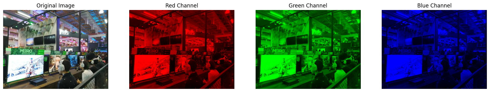
image_path = '/kaggle/working/3.jpg'
image = Image.open(image_path)

image_array = np.array(image)

print(f'Image shape: {image_array.shape}')

fig, ax = plt.subplots(1, 4, figsize=(20, 5))

ax[0].imshow(image_array)
ax[0].set_title('Original Image')
ax[0].axis('off')

channels = ['Red', 'Green', 'Blue']
for i, channel in enumerate(channels):
    single_channel_image = np.zeros_like(image_array)
    single_channel_image[:, :, i] = image_array[:, :, i]
    ax[i + 1].imshow(single_channel_image)
    ax[i + 1].set_title(f'{channel} Channel')
    ax[i + 1].axis('off')

plt.show()Image shape: (750, 1125, 3)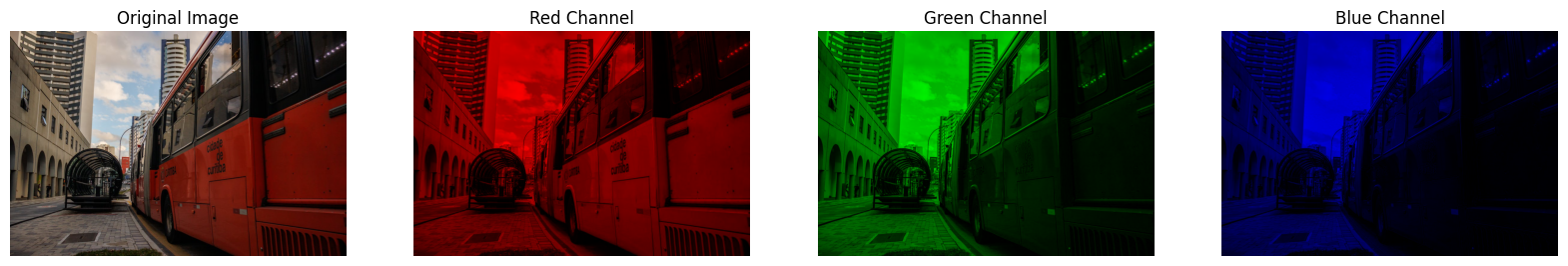
HSV - Hue, Saturation, Value
In the HSV model, the characteristics used to differentiate one color from another are:
- Hue: The dominant color perceived by the observer, representing the base color of the spectrum.
-
Saturation: The intensity or purity of the color, defined by the amount of white light mixed with a color.
- Pure colors from the continuous color spectrum are fully saturated.
- Colors like pink (red and white) and lilac (violet and white) are less saturated, meaning they have a lower intensity of color purity.
- Value: The brightness or intensity of the color, ranging from lighter to darker shades.
import matplotlib.pyplot as plt
import numpy as np
from PIL import Image
from matplotlib.colors import rgb_to_hsv

image_path = '/kaggle/working/2.jpg'
image = Image.open(image_path)

image_array = np.array(image)

print(f'Image shape: {image_array.shape}')

hsv_image = rgb_to_hsv(image_array / 255.0)

fig, ax = plt.subplots(1, 4, figsize=(20, 5))

ax[0].imshow(image_array)
ax[0].set_title('Original Image')
ax[0].axis('off')

channels = ['Hue', 'Saturation', 'Value']
for i, channel in enumerate(channels):
    ax[i + 1].imshow(hsv_image[:, :, i], cmap='gray')
    ax[i + 1].set_title(f'{channel} Channel')
    ax[i + 1].axis('off')

plt.show()Image shape: (750, 1000, 3)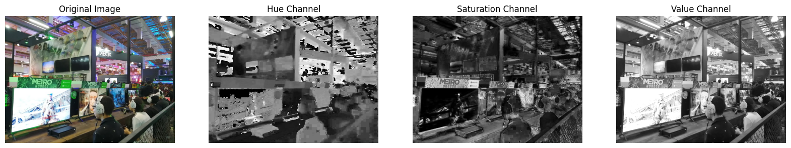
import matplotlib.pyplot as plt
import numpy as np
from PIL import Image
from matplotlib.colors import rgb_to_hsv

image_path = '/kaggle/working/3.jpg'
image = Image.open(image_path)

image_array = np.array(image)

print(f'Image shape: {image_array.shape}')

hsv_image = rgb_to_hsv(image_array / 255.0)

fig, ax = plt.subplots(1, 4, figsize=(20, 5))

ax[0].imshow(image_array)
ax[0].set_title('Original Image')
ax[0].axis('off')

channels = ['Hue', 'Saturation', 'Value']
for i, channel in enumerate(channels):
    ax[i + 1].imshow(hsv_image[:, :, i], cmap='gray')
    ax[i + 1].set_title(f'{channel} Channel')
    ax[i + 1].axis('off')

plt.show()Image shape: (750, 1125, 3)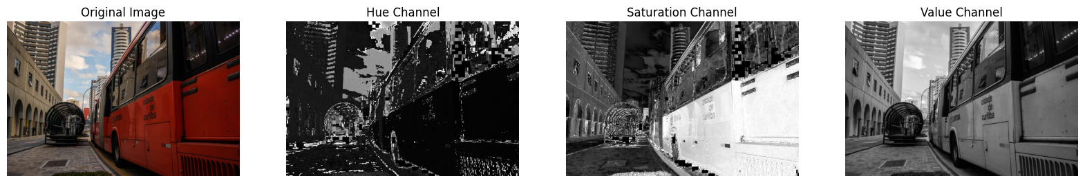
References
Gonzalez, R. C., & Woods, R. E. (2008). Digital image processing (3rd ed.). Pearson Prentice Hall.
Author's notes
Thank you very much for reading this far. If you could like and share, I would be very grateful. If you didn't like it, I can't know if you liked the post. This way, you help me know where I should improve my posts. Thank you.
My Latest Posts


Favorites Projects Open Source
- 🐍 Python
- 🖥️ Deep Learning
- 👀 Computer Vision
- 🖥️ Linux
- 📉 Times Series
- 💾 Database
- 🦀 Rust
- 🖥️ Machine Learning
- 🛣️ Roadmaps
About the author:

A little more about me...
Graduated in Bachelor of Information Systems, in college I had contact with different technologies. Along the way, I took the Artificial Intelligence course, where I had my first contact with machine learning and Python. From this it became my passion to learn about this area. Today I work with machine learning and deep learning developing communication software. Along the way, I created a blog where I create some posts about subjects that I am studying and share them to help other users.
I'm currently learning TensorFlow and Computer Vision
Curiosity: I love coffee