Why ❌ GAN
In the ever-evolving landscape of generative models, GANs have taken center stage with their remarkable ability to generate data that mimics real-world distributions. But as with all great things, classic GANs came with caveats—training instability, vanishing gradients, and mode collapse, to name a few.
Let’s dive deeper into these powerful models: WGAN and its enhanced cousin WGAN-GP, two sophisticated upgrades that fix many of GANs' shortcomings.

What is Wasserstein distance
Wasserstein Distance, also known as the Earth Mover's Distance (EMD), is a mathematical measure of the distance between two probability distributions.
Imagine you have two piles of sand—one symbolizing real data and the other representing data generated by a model. The goal is to reshape one pile into the other by moving portions of sand. The effort required depends not only on how much sand you move but also on how far you move it. This effort is what the Wasserstein Distance measures—a cost-efficient way to transform one distribution into another.
What makes this distance especially powerful is its ability to compare distributions even when they don't overlap at all—a situation where traditional measures like JS divergence fail. It offers a continuous and interpretable signal for how "far off" the generated data is from the real data, making it incredibly useful for training generative models like WGANs.
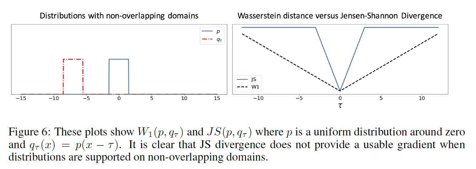
Traditional GANs use Jensen-Shannon (JS) divergence to measure similarity between distributions.
BUT :
- JS divergence becomes undefined or uninformative when distributions don't overlap.
- This leads to vanishing gradients—a huge problem for training
By contrast, Wasserstein Distance:
- Remains well-defined and continuous even when distributions are far apart.
- Provides meaningful gradients, allowing the generator to learn effectively from the start.
Improvement in WGAN wrt GAN
WGAN is a variant of GAN that uses the Wasserstein Distance as its loss function instead of JS divergence.
Key differences from traditional GAN:
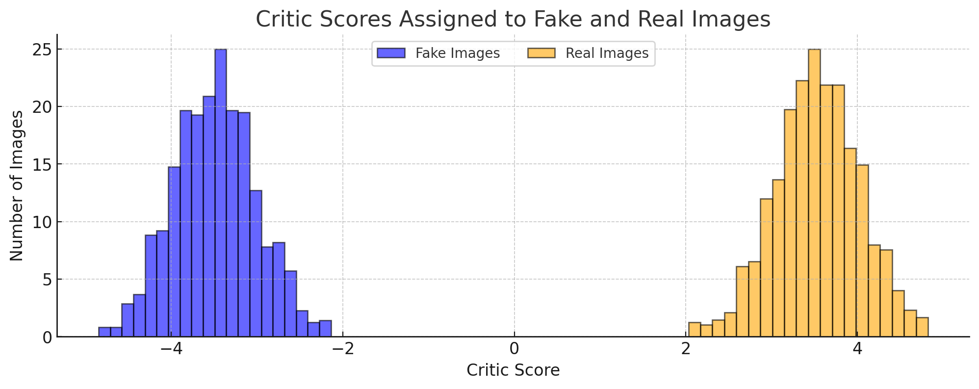
The discriminator is now called a critic. It doesn't classify data as real/fake, but scores it to reflect how “real” it looks.
The loss function is based on the difference in critic scores for real vs. fake data.
In simple terms:
Real Data → High Critic Score
Fake Data → Low Critic Score
The generator improves by producing data that the critic scores higher.
Working
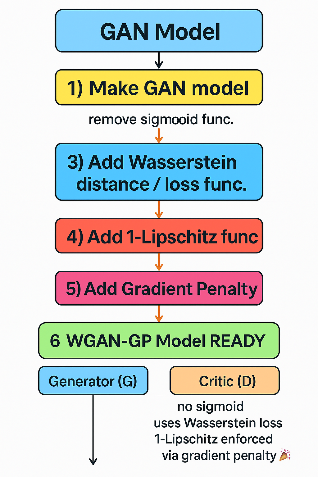
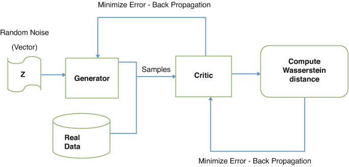
Just like in standard GANs, WGAN consists of two neural networks:
A Generator (G) that tries to generate realistic data from random noise.
A Critic (C) (not called a discriminator here) that scores the realness of data, assigning higher values to real data and lower values to fake ones.
Unlike GANs, which use a sigmoid function to classify samples as real or fake, WGAN's critic outputs real-valued scores—this small shift changes everything.
The Loss Function
The heart of WGAN lies in replacing Jensen-Shannon divergence with the Wasserstein distance (also called Earth Mover’s Distance)—a metric that measures how much "effort" it takes to morph the generated distribution into the real one.
This results in the following loss functions:
Critic's Loss:
𝐿c = E[C(fake)]−E[C(real)]
The critic aims to maximize the difference, rewarding real data with higher scores and penalizing fakes.
Generator's Loss:
𝐿G = −E[C(fake)]
The generator tries to minimize the critic’s ability to detect its fakes by generating better, more realistic data.
Missing Something? 🤔
The model that we learned until now has some issues.
-
The critic assigns real-valued scores to data samples, so nothing stops the critic from amplifying its outputs to maximize the loss. For example, it might assign real samples a score of +10,000. And fake samples a score of -10,000. This leads to :
- The generator receiving extreme gradients, which are not helpful and can distort learning.
- Loss curves spike or crash. Generated samples look worse over time instead of better, making training unstable.
- Mode collapse and exploding gradients can occur.
How can we solve this problem?
Let's introduce a 1-Lipschitz Function. This will solve our problem.
We will add a 1-Lipschitz Function to the critic (discriminator).
In the Lipshitz function, we will give any 2 images (x1 and x2) as input.
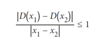
Numerator: Absolute difference between the critic predictions
Denominator: Average pixelwise absolute difference between two images.
What we are trying to do with this function is to limit the rate at which the predictions of the critic can change between 2 images, when comparing it with the real/pixel-wise difference of the image.
You can get this using a graph by visualizing 2 (white) cones whose origin can be moved along the graph so that the whole graph always stays outside the cones.
By doing so, we are clipping the weights of the critic to lie within a small range, eliminating problems of exploding gradients.
But again NEW PROBLEM !!
Learning significantly decreases 😢 😢
A much better Solution is the WGAN-GP
Adding Gradient Penalty
As the Lipshitz function did a partial job. We need to modify/tweak the function so that it can eliminate the problem of Learning significantly decreases.
The solution should be to penalize the Gradient if it's too far away from 1.
The Lipschitz constraint is enforced by including a gradient penalty (GP) term in the loss function for the critic. The GP penalizes the model if the gradient norm deviates from 1
The GP term, which we will be using with Lipschitz constraint, will measure the square difference between the gradient of the prediction wrt input image and 1.
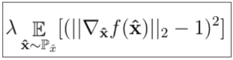
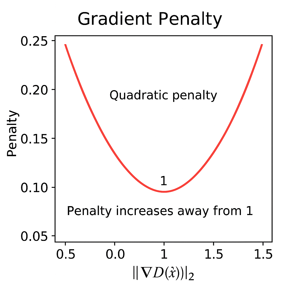
From the above image, it's clear that the gradient penalty increases as we move away from 1.
There are a few important things to take care of while using training WGAN-GP :
With Wasserstein loss, the Critic must be trained to converge before updating the Generator. To do so, we train the Critic several times between Generator updates. A typical ratio used is
3 to 5 Critic updates per Generator update.Batch Normalization shouldn't be used in the critic. Batch Norm creates a correlation between images in the same batch. This makes the gradient penalty loss less effective. Experiments have shown that WGAN-GPs works great without it anyway
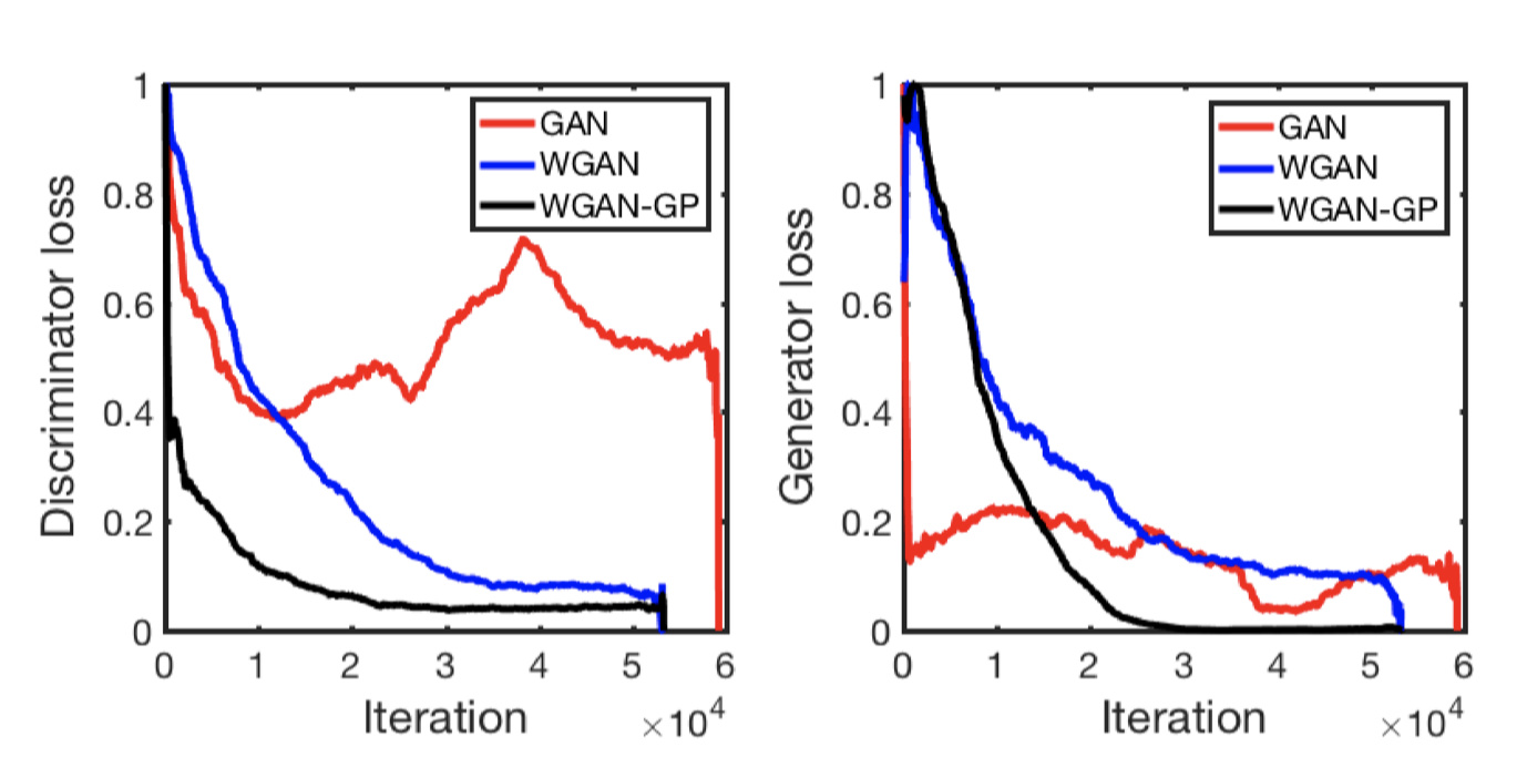
Results after WGAN-GP model:
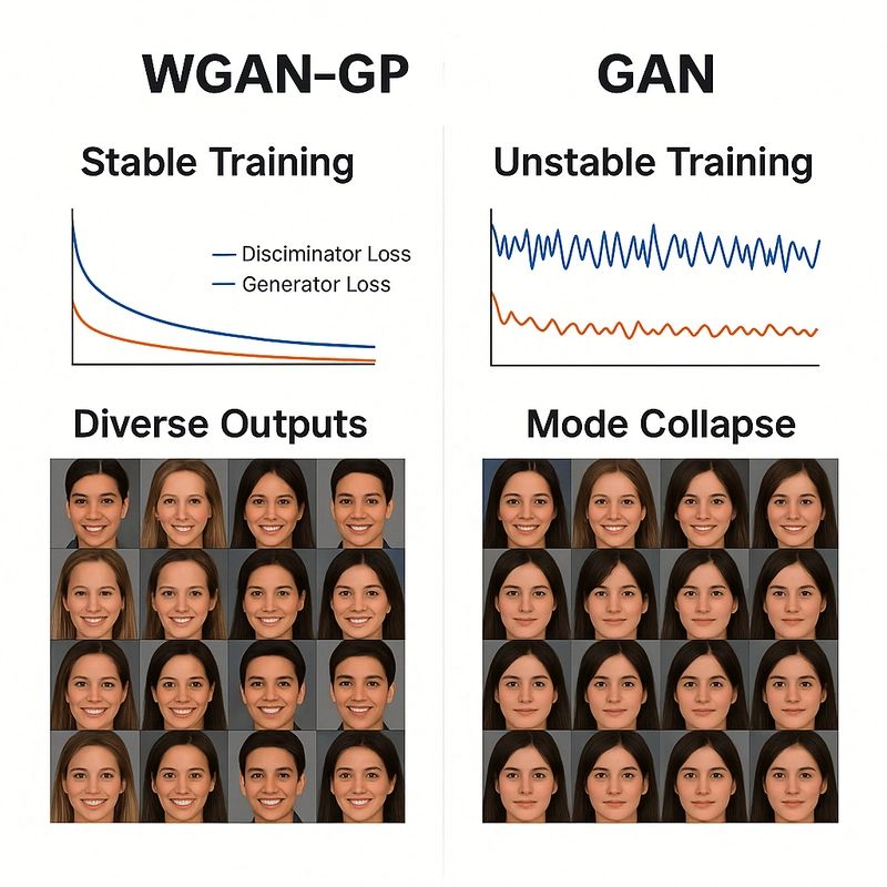
Using Wasserstein distance + Lipschitz function + Gradient penalty has improved the results of the images generated significantly.
- Traditional GANs suffer from vanishing gradients or mode collapse due to the Jensen-Shannon divergence. WGAN-GP, by using Wasserstein distance + gradient penalty, leads to more consistent and stable convergence. You get smoother generator updates, making training less sensitive to hyperparameters and architectural choices.
- In classic GANs, generators can produce a limited variety (mode collapse). WGAN-GP encourages the generator to explore the data distribution more fully, thanks to the meaningful gradient feedback from the critic. Hence, more diverse outputs, especially noticeable in image generation tasks.
- The loss correlates with sample quality, unlike traditional GAN loss, which becomes meaningless when the discriminator is too good. Hence, you can track training progress numerically, not just visually
- There are no sudden spikes or flat zones in gradients. Hence, more efficient and productive generator learning.
Disadvantages of WGAN
Slower training, higher memory usage, and increased training time, especially on large datasets.
Hyperparameters are sensitive. Even a small change in hyperparameters can cause a lot of change. It needs to be tuned carefully.
Summarize
- A WGAN-GP uses the Wasserstein loss
- The WGAN-GP is trained using labels of 1 for real and -1 for fake
- No Sigmoid activation in the final layer of the Critic
- Include a GP term in the loss function for the Critic
- Train the Critic multiple times for each update of the Generator
- There are no Batch Norm layers in the Critic