Have you ever played Outer Wilds? The planets there are incredibly beautiful. This actually became the main motivation to create my own simple model of a planet, using real geographical elevation data and a bit of Wolfram Language magic.
TL;DR; Here is an interactive animation
Notes on IDE
In this tutorial, I (@jerryi) am going to use an open-source notebook interface, WLJS Notebook, based on the freeware Wolfram Engine.
Spreading points on a sphere
Obviously, even if we grab Earth's elevation map, there’s the problem of projecting it onto a sphere. This is a complex topic involving triangulation (since we need to create polygons from it afterward) and more, with plenty written on the subject. For example:
As one approach, we’ll go the other way around—first generating sample points on the sphere, then querying the elevation data for those points.
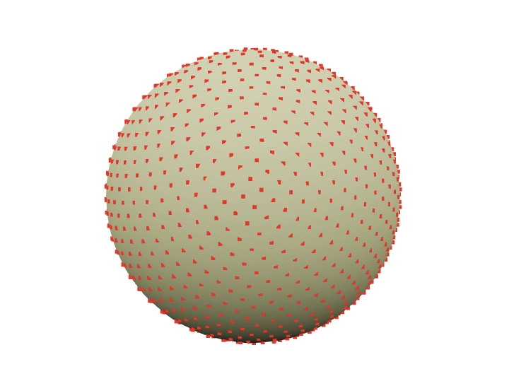
So, we need to evenly distribute N points across a sphere. No need to reinvent the wheel when a rich standard library is available.
Graphics3D[{
  Sphere[],
  Red, PointSize[0.01], SpherePoints[1000]//Point
}]
Get Elevation Data
Fortunately (or unfortunately), the standard WL library already includes a rough map of the entire Earth (just in case). If more precision is needed, it can go online and fetch higher-resolution data.
So, let’s get down to business
GeoElevationData[GeoPosition[Here]]output
Quantity[490, "Meters"]Here, Here returns the current latitude and longitude in degrees. The function can take not just a single value but an entire list. Naturally, we’ll use this list from the points on the sphere.
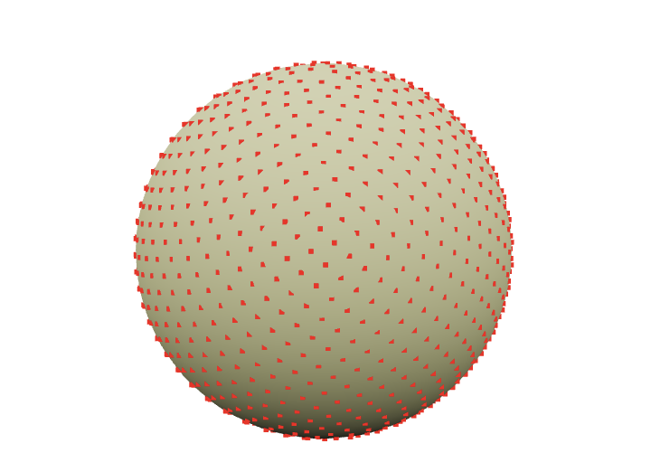
points = SpherePoints[5000];
latLon = (180/Pi) {90Degree - ArcCos[#[[3]]], ArcTan[#[[1]], #[[2]]]} &/@ points;
elevation = GeoElevationData[GeoPosition[latLon]];
elevation = (elevation + Min[elevation])/Max[elevation];
Here we convert from Cartesian coordinates to spherical (more precisely, geodetic) coordinates

we retrieve the elevations and normalize them.
The final step is to link them back to the original points on the sphere, using the normalized elevation as the distance along the normal.
surface = MapThread[(#1 (0.8 + 0.1 #2))&, {points, elevation}];Here, we scale them by eye so that the height above sea level only slightly "modulates" the sphere’s surface. This way, we get a visible relief of the Earth
rainbow = ColorData["DarkRainbow"];

ListSurfacePlot3D[surface,
  Mesh->None, MaxPlotPoints->100,
  ColorFunction -> Function[{x,y,z},
      rainbow[1.5(2 Norm[{x,y,z}]-1)]
  ], ColorFunctionScaling -> False
]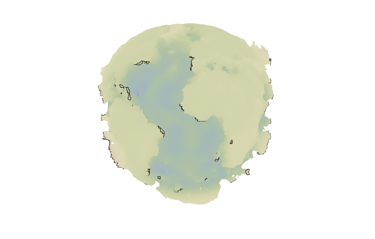
That looks like Earth!
Generating clouds
What’s Earth without clouds? And what are clouds without Perlin noise?
The next piece I honestly stole from one of the forums (no GPT for you!)
n = 128;
k2 = Outer[Plus, #, #] &[RotateRight[N@Range[-n, n - 1, 2]/n, n/2]^2];

spectrum = With[{d := RandomReal[NormalDistribution[], {n, n}]},
   (1/n) (d + I d)/(0.002 + k2)];
spectrum[[1, 1]] *= 0;

im[p_] := Clip[Re[InverseFourier[spectrum Exp[I p]]], {0, ∞}]^0.5

p0 = p = Sqrt[k2];

Image[im[p0 += p], Magnification->2]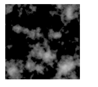
Here animated version
Module[{buffer = im[p0 += p], frame = CreateUUID[]},
  EventHandler[frame, (buffer = im[p0 += p])&];

  Image[buffer // Offload,
    Magnification->2,
    Epilog->AnimationFrameListener[buffer // Offload, "Event"->frame]
  ]
]
How do we make them three-dimensional? I couldn’t think of anything better than using the Marching Cubes technique to generate low-poly clouds.
However, to start, we’ll "stretch" the 2D image into 3D with fading at the edges.
With[{plain = im[p0+=p]}, Table[plain Exp[-( i)^2/200.], {i, -20,20}]][[;;;;8, ;;;;8, ;;;;8]] // Image3D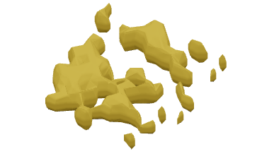
To turn this scalar field into polygons, we can use the ImageMesh function. However, it's quite challenging to work with when nonlinear transformations need to be applied to the mesh. And we will need to do these transformations, otherwise, how will we map this square onto the sphere?
Let’s use an external library, wl-marchingcubes.
PacletRepositories[{
    Github -> "https://github.com/JerryI/wl-marching-cubes" -> "master"
}]

<<JerryI`MarchingCubes`With[{plain = im[p0+=p]}, Table[plain Exp[-( i)^2/200.], {i, -20,20}]];
{vertices, normals} = CMarchingCubes[%, 0.2];The result is stored in vertices. By default, the library generates an unindexed set of triangle vertices. This means we can directly interpret them as
Polygon[{
  {1, 2, 3},  Triangle 1
  {4, 5, 6},  Triangle 2
  ...
}]
Where none of the vertices are reused by another triangle. This format is especially simple for the GPU, as only one such list needs to be sent to one of the WebGL buffers. Fortunately, our (WLJS Notebook) implementation of Polygon primitive supports this format unlike Wolfram Mathematica
GraphicsComplex[vertices, Polygon[1, Length[vertices]]] // Graphics3D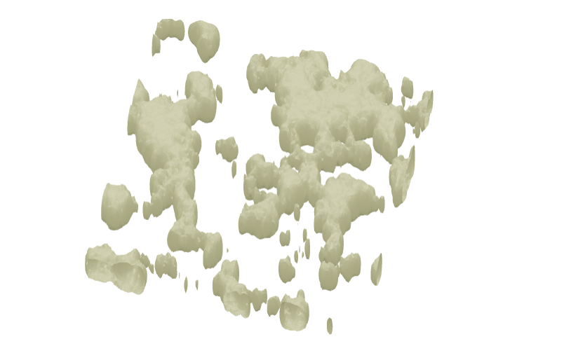
Inverse UV-mapping
It is important to note, that on the next few steps we will map those clouds on the sphere (our Earth surface model). The easiest way is to perform so-called UV-mapping, which will naturally distort our original texture. Especially on poles.
For the educational purpose let's perform a naive inverse UV-mapping (from the the "texture" to a sphere)

where

Those 3 coordinates are vertices of generated clouds normalized in the range from 0 to 1 (except 3rd one)
With[{plain = im[p0 += p]}, Table[plain Exp[-( i)^2/200.], {i, -20,20}]];

{vertices, normals} = CMarchingCubes[%, 0.2, "CalculateNormals" -> False];

vertices = With[{
  offset = {Min[vertices[[All,1]]], Min[vertices[[All,2]]], 0},
  maxX = Max[vertices[[All,1]]] - Min[vertices[[All,1]]],
  maxY = Max[vertices[[All,2]]] - Min[vertices[[All,2]]]
}, Map[Function[v, With[{p = v - offset}, {p[[1]]/maxX, p[[2]]/maxY, p[[3]]}]], vertices]];

pvertices = Map[Function[v,
    With[{\[Rho] = 50.0 + 0.25 (v[[3]] - 10), \[Phi] =  2 Pi Clip[v[[1]], {0,1}], \[Theta] =  Pi Clip[v[[2]], {0,1}]},
      {\[Rho] Cos[\[Phi]] Sin[\[Theta]], \[Rho] Sin[\[Phi]] Sin[\[Theta]], \[Rho] Cos[\[Theta]]}
    ]
  ]
, vertices];

{
  GraphicsComplex[0.017 pvertices, Polygon[1, Length[vertices]]]
} // Graphics3D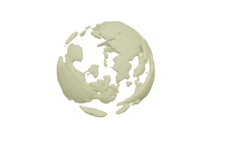
This looks horrible on the poles 👎
There are two problems to solve
- distortions on poles
- incorrect aspect ratio of "clouds"
We need to go back and rethink our approach.
Correcting aspect ratio
This is relatively easy to fix, we need a rectangle with 1/2 ratio
n = 256;
ratio = 1/2;

k2 = Outer[Plus, #, #] &[RotateRight[N@Range[-n, n - 1, 2]/n, n/2]^2];

k2 = k2[[;; ;; 1/ratio, All]];

spectrum = With[{d := RandomReal[NormalDistribution[], {n ratio, n}]},
   (1/n) (d)/(0.001 + k2)];
spectrum[[1, 1]] *= 0;

im[p_] := Clip[Re[InverseFourier[spectrum Exp[I p]]], {0, ∞}]^0.5

p0 = p = Sqrt[k2];

cloudTexture = im[p0 += p] // Image;
Double check if it is still repeating from all 4 sides
Table[cloudTexture, {2}, {2}] // Grid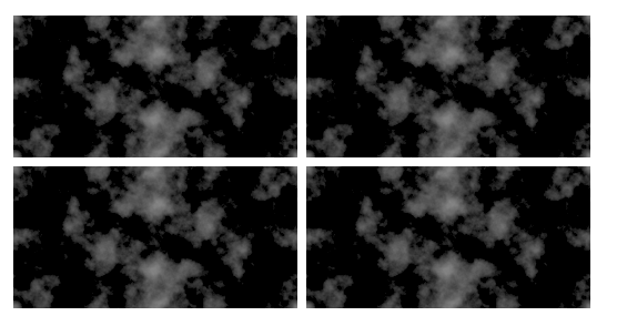
There is a 🚀 science behind the question how to project things on or from the sphere
Mapping things to a sphere
I'll mention right away that I’m not an expert in geodesy (@jerryi ), but I’ve "heard" about some concepts from computational geometry and 3D graphics ;)
In any case, we’ll be "mapping" this texture onto the sphere in one form or another (as polygons). This means we’ll transform all its points following one of the cartographic projections.
A method we used UV-mapping is analogous to an equal-area cartographic projection, with the exception of coefficients responsible for angle shifts.
Let’s imagine that if we apply some inverse transformation to our original texture, when projecting it onto the sphere, they should compensate for each other, and we’ll see an undistorted image of the clouds.
Then, the questions are:
What is our original texture right now, and what do we want to see in the end?
What does an undistorted image mean in this context?
How can we generally talk about what we want to see on the sphere while looking at a rectangular Perlin noise image in Cartesian coordinates?
These questions could be answered in this article if I were an expert in the subject 🧐 Unfortunately, I cannot meet that criterion, so let's at least try to find a way to eliminate artifacts at the poles. Looking at textures from games, we can notice a pattern
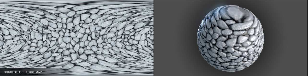
https://richardrosenman.com/shop/spherical-mapping-corrector/
At the edges of the texture projected from the sphere, the details stretch towards the top and bottom edges of the rectangle. This is exactly the case of our poles.
Thus, if we artificially distort the original texture in the same way, we should eliminate the artifacts at the poles. Do you know what this transformation resembles?
It’s akin to transforming the Mollweide projection into an equal-area cartographic projection
lat[y_, rad_:1] := ArcSin[(2 theta[y, rad] + Sin[2 theta[y, rad]])/Pi];
lon[x_, y_, rad_:1, lonzero_: 0] := lonzero + Pi x/(2 rad Sqrt[2] Cos[theta[y, rad]]);
theta[y_, rad_:1] := ArcSin[y/(rad Sqrt[2])];
mollweidetoequirect[{x_, y_}] := {lon[x, y, 1], lat[y]};

newCloudTexture = ImageForwardTransformation[
  cloudTexture,
  mollweidetoequirect,
  DataRange -> {{-2 Sqrt[2], 2 Sqrt[2]}, {-Sqrt[2], Sqrt[2]}},
  PlotRange -> All
];

Image[%, Magnification->2]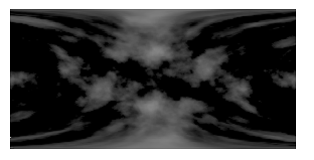
Next, we simply need to repeat Marching Cubes on it and transform all the vertices using the equation above. As a bonus, let's transform normals as well!
With[{plain = ImageData[newCloudTexture]}, Table[plain Exp[-( i)^2/200.], {i, -20,20}]];

{vertices, normals} = CMarchingCubes[%, 0.2];

vertices = With[{
  offset = {Min[vertices[[All,1]]], Min[vertices[[All,2]]], 0},
  maxX = Max[vertices[[All,1]]] - Min[vertices[[All,1]]],
  maxY = Max[vertices[[All,2]]] - Min[vertices[[All,2]]]
}, Map[Function[v, With[{p = v - offset}, {p[[1]]/maxX, p[[2]]/maxY, p[[3]]}]], vertices]];

{pvertices, pnormals} = MapThread[Function[{v,n},
    With[{\[Rho] = 50.0 + 0.25 (v[[3]] - 10), \[Phi] =  2 Pi Clip[v[[1]], {0,1}], \[Theta] =  Pi Clip[v[[2]], {0,1}]},
      {
        {\[Rho] Cos[\[Phi]] Sin[\[Theta]], \[Rho] Sin[\[Phi]] Sin[\[Theta]], \[Rho] Cos[\[Theta]]},

        n[[3]] {Cos[\[Phi]] Sin[\[Theta]], Sin[\[Phi]] Sin[\[Theta]], Cos[\[Theta]]} +
        n[[2]] {Cos[\[Theta]] Cos[\[Phi]],Cos[\[Theta]] Sin[\[Phi]],-Sin[\[Theta]]} +
        n[[1]] {-Sin[\[Theta]] Sin[\[Phi]],Cos[\[Phi]] Sin[\[Theta]],0}
      }
    ]
  ]
, {vertices, -normals}] // Transpose;

{
  clouds = GraphicsComplex[0.017 pvertices, Polygon[1, Length[vertices]], VertexNormals->pnormals]
} // Graphics3D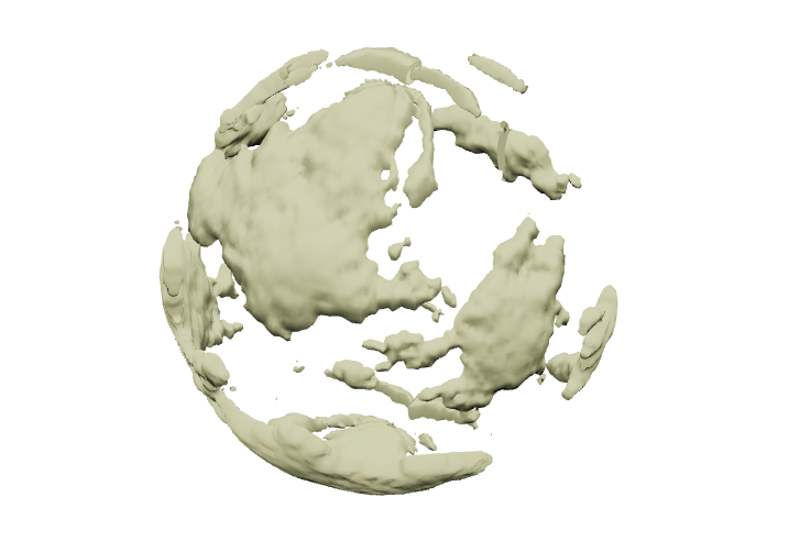
If VertexNormals is explicitly set in GraphicsComplex, then when shading, the surface will be interpolated across all three normals of the triangle, instead of just one (which is automatically calculated by the graphics library if no other data is provided, in which case the polygon looks like a flat plane — a.k.a. the effect seen in 80s demos).
Putting it all together
We can extend the original SurfacePlot with options and add additional graphic primitives through them. Oh, and don’t forget to turn off the default lighting. After all, we’re in space!
rainbow = ColorData["DarkRainbow"];

ListSurfacePlot3D[
  MapThread[(#1 (0.8 + 0.1 #2))&, {points, elevation}],
  Mesh->None, MaxPlotPoints->100,
  ColorFunction -> Function[{x,y,z}, rainbow[1.5(2 Norm[{x,y,z}]-1)]],
  ColorFunctionScaling -> False,
  Lighting->None,
  PlotStyle->Directive["Shadows"->True, "CastShadow"->True],

  Prolog -> {
    Directive["Shadows"->True, "CastShadow"->True],
    clouds,
    HemisphereLight[LightBlue, Orange // Darker // Darker],
    SpotLight[Orange, {-2.4909, 4.069, 3.024}]
  },

  Background->Black
, ImageSize->800]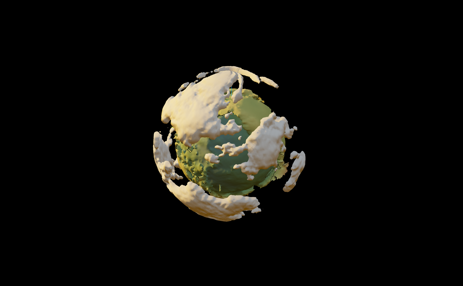
We can play around with real-time lighting by adding a handler to the transform property of a small sphere at the light source’s position
rainbow = ColorData["DarkRainbow"];
lightPos = {-2.4909, 4.069, 3.024};


ListSurfacePlot3D[
  MapThread[(#1 (0.8 + 0.1 #2))&, {points, elevation}],
  Mesh->None, MaxPlotPoints->100,
  ColorFunction -> Function[{x,y,z}, rainbow[1.5(2 Norm[{x,y,z}]-1)]],
  ColorFunctionScaling -> False,
  Lighting->None,
  PlotStyle->Directive["Shadows"->True, "CastShadow"->True],

  Prolog -> {
    Directive["Shadows"->True, "CastShadow"->True],
    clouds,
    HemisphereLight[LightBlue, Orange // Darker // Darker],
    SpotLight[Orange, lightPos // Offload],
    EventHandler[Sphere[lightPos, 0.001], {"transform" -> Function[t,
      lightPos = t["position"]
    ]}]
  },

  Background->Black
, ImageSize->800]
Animation
Let’s add a simple animation for the movement of the light source, as well as the rotation of the cloud sphere to spice up the scene using a single slider
rainbow = ColorData["DarkRainbow"];
lightPos = {-2.4909, 4.069, 3.024};

rotationMatrix = RotationMatrix[0., {0,0,1}];

EventHandler[InputRange[0,1, 0.01], Function[value,
  lightPos = RotationMatrix[2Pi value, {1,1,1}].{-2.4909, 4.069, 3.024} // N;
  rotationMatrix = RotationMatrix[2Pi value, {0,0,1}] // N;
]]

ListSurfacePlot3D[
  MapThread[(#1 (0.8 + 0.1 #2))&, {points, elevation}],
  Mesh->None, MaxPlotPoints->100,
  ColorFunction -> Function[{x,y,z}, rainbow[1.5(2 Norm[{x,y,z}]-1)]],
  ColorFunctionScaling -> False,
  Lighting->"Default",
  PlotStyle->Directive["Shadows"->True, "CastShadow"->True],

  Prolog -> {
    Directive["Shadows"->True, "CastShadow"->True],
    GeometricTransformation[clouds, rotationMatrix // Offload],
    HemisphereLight[LightBlue, Orange // Darker // Darker],
    SpotLight[Orange, lightPos // Offload]
  },

  Background->Black,
  ImageSize->800
]
Try it by yourself
Here is a web-version of this notebook and it is fully interactive 🧙🏼♂️