This is a Plain English Papers summary of a research paper called Smarter Time-Series: AI Adapts Forecasts to Your Specific Needs. If you like these kinds of analysis, you should join AImodels.fyi or follow us on Twitter.
Introduction: The Need for Context-Aware Forecasting
Traditional time-series forecasting (TSF) models typically focus on minimizing prediction errors across the entire value range. This approach ignores a crucial reality: in real-world applications, the importance of accurate predictions varies dramatically depending on the specific value ranges that matter to downstream tasks.
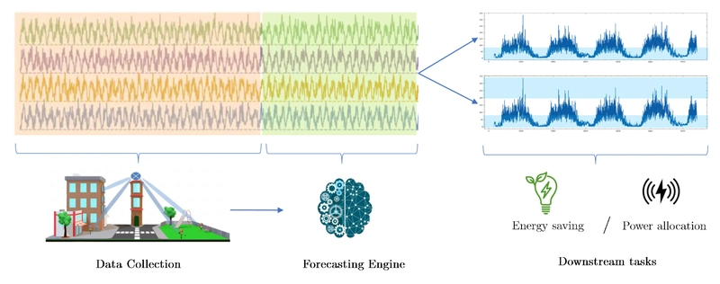
For example, in wireless network management, different applications have completely different requirements. Energy efficiency protocols need accurate forecasts primarily during low-traffic periods to optimize base station deactivation, while power allocation algorithms require precision at both high and low traffic extremes.

This figure illustrates how different wireless network applications require accuracy in different value ranges. Energy efficiency needs precision during low traffic, while power allocation needs accuracy at both high and low extremes.
This research introduces a groundbreaking training methodology that allows forecasting models to dynamically adjust their focus based on the importance of specific value ranges specified by the end application. Unlike previous methods that fix these ranges beforehand, this approach breaks down predictions into smaller segments that can be dynamically weighted and combined at inference time.
Recent advances in time-series forecasting have produced powerful foundation models like Timer, Moirai, TimesFM, Chronos, Moment, and Toto. This work builds upon these advances by creating a framework that better connects prediction to decision-making in practical applications.
Literature Review: Advances in Time-Series Forecasting
The time-series forecasting landscape has evolved dramatically from statistical methods like ARIMA and Exponential Smoothing to sophisticated deep learning approaches. Recent years have seen particularly rapid advancement in adapting Transformer architectures for time-series data.
Key developments in Transformer-based forecasting include:
- Refining attention mechanisms for temporal data
- Transforming input token representations through techniques like stationarization and patching
- Broadly modifying the Transformer architecture and its modules
The iTransformer represents a significant breakthrough in this space by inverting the traditional Transformer approach to better handle time-series data.
Simultaneously, research has explored customizing objective functions for specific forecasting needs. Some works focus on integrating uncertainty quantification or fairness considerations, while others derive loss weights from downstream task characteristics. The current research distinguishes itself by enabling a single model to accommodate diverse downstream requirements at inference time rather than training time.
The Forecasting Problem: Mathematical Formulation
A multivariate time-series consists of vector-valued observations ordered temporally. Let x₍ₜ₎ ∈ ℝⁿ denote an n-dimensional real-valued vector observed at time t, where t ∈ [T] and n ≥ 1. The full time-series is represented as the ordered set {x₍₁₎, x₍₂₎, ..., x₍ₜ₎}.
Time-series forecasting is reformulated as a supervised regression task by constructing input-output pairs from sliding windows over the series. With forecast horizon τ and window size w, for each time t, the input X₍ₜ₎ = x₍ₜ₋ᵥ:ₜ₋₁₎ consists of a history window {x₍ₜ₋ᵥ₎, ..., x₍ₜ₋₁₎}, and the target Y₍ₜ₎ = x₍ₜ:ₜ₊τ₋₁₎ is the future window {x₍ₜ₎, ..., x₍ₜ₊τ₋₁₎}.
The learning problem involves finding a mapping f(X) parameterized by θ to approximate the underlying dynamics Y = f(X) + ε, where ε is noise. The goal is to learn the model θ* that minimizes the expected loss. For task-specific forecasting, this is extended to focus on particular value intervals of interest.
Methodology: Five Approaches to Adaptive Forecasting
This research investigates five progressively more sophisticated approaches to create models that can adapt to varying value intervals at inference time:
Baseline Policy (B-Policy): Standard approach that doesn't incorporate interval sensitivity.
Task-specific Policy (E2E-Policy): Optimizes for a single predefined interval of interest, making it ideal for specific applications but not adaptable.
Continuous-Interval Training Policy (C-Policy): Incorporates the target interval as a covariate, training the model to handle any interval within the value range.
Discrete-Interval Training Policy (D-Policy): Trains on a finite set of predefined intervals, creating a more manageable learning problem.
Enhanced D-Policy with Interval Patching: Combines predictions from multiple intervals using either averaging (D¹ₗ-Policy) or maximum selection (D∞ₗ-Policy) strategies.
The weighing mechanism for values inside target intervals is illustrated below:
![a) The weighing mechanism for values inside interval [0.25, 0.5] with a large decay rate ν→∞.](/uploads/2025/05/68175b26d03bc.png)
The weighing mechanism for values inside interval [0.25, 0.5] with a large decay rate approaching infinity, creating sharp boundaries.
![b) The weighing mechanism for values inside interval [0.25, 0.5] with decay rate ν=37.](https://media2.dev.to/dynamic/image/width=800%2Cheight=%2Cfit=scale-down%2Cgravity=auto%2Cformat=auto/https%3A%2F%2Fdev-to-uploads.s3.amazonaws.com%2Fuploads%2Farticles%2Fjg5sny80qtq6scpt0lye.png)
The weighing mechanism for values inside interval [0.25, 0.5] with a moderate decay rate of 37, creating smoother transitions at interval boundaries.
The most advanced approach, the adaptive interval policy, leverages discrete interval training and incorporates a classifier that helps selectively utilize interval-specific forecasts. This achieves flexibility across arbitrary target intervals, enabling a single model to adapt to different downstream tasks during inference.
Experiments: Testing the Framework
Experimental Setup
The experiments employed four state-of-the-art models: iTransformer, DLinear, PatchTST, and TimeMixer. Each model was modified to integrate target interval information:
- For iTransformer, the interval representation was concatenated to the temporal encoding tensor
- For other models, the interval values were processed as auxiliary temporal channels
To evaluate dual-task objectives (both forecasting and interval classification), each model was augmented with a classification head by doubling the final projection layer.
The research used several datasets:
- SynthDS: A synthetic dataset designed to highlight the methodology's components
- BLW-TrafficDS: A real-world wireless network traffic dataset
- Standard benchmark datasets including ETTh1, ETTh2, ETTm1, and ETTm2
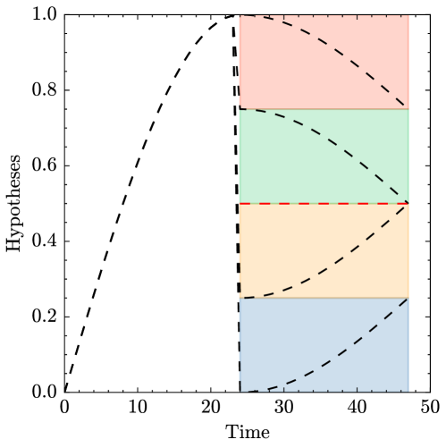
The noise-free hypotheses used to construct the synthetic trace SynthDS, showing multiple possible patterns.

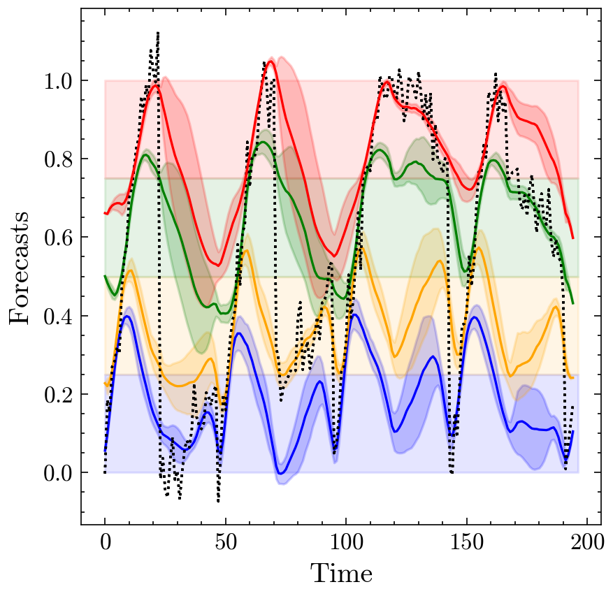
The baseline model (B-Policy) converges to predicting the average hypothesis (red line at 0.5), highlighting its inability to distinguish between different patterns in the data.
Numerical Results
The baseline policy (B-Policy) exhibited clear averaging behavior, converging to the midpoint of the trace in SynthDS. This demonstrates a critical limitation: standard approaches can't differentiate between different value patterns when they have similar statistical properties.
Models trained with E2E-Policy on four different intervals of interest, showing how end-to-end training enables targeting specific value ranges.
The C-Policy evaluated on four different intervals, showing its ability to adapt to different value ranges but with lower accuracy than specialized policies.

The impact of interval-separation percentage (δ) on performance, showing that while performance improves as sampling space support is reduced, it eventually degrades when exceeding the true underlying interval length.
The end-to-end training policy (E2E-Policy) demonstrated excellent performance when configured for specific intervals but lacked adaptability. The continuous policy (C-Policy) provided adaptability but struggled to capture the relationship between intervals and their hypotheses accurately.
The discrete interval policies (D-Policy and its enhanced variants) achieved the best balance of accuracy and adaptability:
| Model | Training Strat. | $\mathcal{I}_{1}$ | $\mathcal{I}_{2}$ | $\mathcal{I}_{3}$ | $\mathcal{I}_{4}$ | $\mathcal{I}_{5}$ | $\mathcal{I}_{6}$ | $\mathcal{I}_{7}$ | $\mathcal{I}_{8}$ | Avg. |
|---|---|---|---|---|---|---|---|---|---|---|
| DLinear | $\mathrm{D}_{9}$-Policy | 167.1 | 76 | 56.7 | 44.2 | 33.5 | 28.1 | 19.3 | 11.1 | 54 |
| $\mathrm{D}_{16}^{*}$-Policy | 172.3 | 74.9 | 56 | 43.8 | 33.4 | 27.9 | 19.2 | 11.1 | 54.8 | |
| $\mathrm{D}_{16}^{*}$-Policy | 164.9 | 75.7 | 56.7 | 44.4 | 33.8 | 28.2 | 19.4 | 11.2 | 54.3 | |
| B-Policy | 163.8 | 82.4 | 62 | 48.9 | 37.6 | 31.8 | 21.7 | 12.5 | 57.6 | |
| $\mathrm{C}_{0.1}$-Policy | 218 | 84.8 | 58.8 | 43.4 | 31.7 | 26.4 | 18.8 | 10.9 | 61.6 | |
| Improvement | $0.0 \%$ | $9.1 \%$ | $9.7 \%$ | $11.2 \%$ | $15.7 \%$ | $16.9 \%$ | $13.4 \%$ | $12.8 \%$ | $6.3 \%$ | |
| TimeMixer | $\mathrm{D}_{9}$-Policy | 127.5 | 40.1 | 24.3 | 16.1 | 10.8 | 8 | 5.5 | 3.3 | 29.4 |
| $\mathrm{D}_{16}^{*}$-Policy | 148.1 | 37.8 | 22.9 | 15.4 | 10.2 | 7.8 | 5.5 | 3.5 | 31.4 | |
| $\mathrm{D}_{16}^{*}$-Policy | 138 | 41.7 | 23.8 | 15.8 | 10.4 | 8 | 5.6 | 3.4 | 30.9 | |
| B-Policy | 125.9 | 83 | 64.9 | 48.1 | 35.8 | 30.2 | 21.8 | 12.1 | 52.7 | |
| $\mathrm{C}_{0.1}$-Policy | 143.7 | 50.7 | 32 | 20.8 | 13.1 | 9.3 | 6.1 | 3.6 | 34.9 | |
| Improvement | $0.0 \%$ | $54.5 \%$ | $64.7 \%$ | $68.0 \%$ | $71.5 \%$ | $74.2 \%$ | $74.8 \%$ | $72.7 \%$ | $44.2 \%$ | |
| iTransformer | $\mathrm{D}_{9}$-Policy | 119.3 | 74.7 | 57.1 | 44 | 31.4 | 25.2 | 19.2 | 11.2 | 47.8 |
| $\mathrm{D}_{16}^{*}$-Policy | 121.1 | 75.9 | 58.4 | 44.6 | 32.1 | 25.7 | 19.5 | 11.2 | 48.6 | |
| $\mathrm{D}_{16}^{*}$-Policy | 122.8 | 75.7 | 57.6 | 44.1 | 31.9 | 25.7 | 19.5 | 11.2 | 48.6 | |
| B-Policy | 130.8 | 77.3 | 59.5 | 46.8 | 35.5 | 29.8 | 20.6 | 11.8 | 51.5 | |
| $\mathrm{C}_{0.1}$-Policy | 133.1 | 75.6 | 56 | 42.1 | 28.7 | 23.3 | 18.1 | 11.4 | 48.5 | |
| Improvement | $8.8 \%$ | $3.4 \%$ | $5.9 \%$ | $10.0 \%$ | $19.2 \%$ | $21.8 \%$ | $12.1 \%$ | $5.1 \%$ | $7.2 \%$ | |
| PatchTST | $\mathrm{D}_{9}$-Policy | 102.8 | 31.1 | 18.3 | 11.4 | 7.1 | 4.5 | 2.7 | 1.7 | 22.4 |
| $\mathrm{D}_{16}^{*}$-Policy | 158.2 | 30.4 | 17.2 | 10.4 | 6.5 | 4 | 2.4 | 1.5 | 28.8 | |
| $\mathrm{D}_{16}^{*}$-Policy | 117.8 | 35.3 | 20.8 | 12.6 | 7.9 | 5 | 2.8 | 1.8 | 25.5 | |
| B-Policy | 124.1 | 77.9 | 60.3 | 47.2 | 34.9 | 29.4 | 20.4 | 11.7 | 50.7 | |
| $\mathrm{C}_{0.1}$-Policy | 118.1 | 34.6 | 22.5 | 15.2 | 9.8 | 6.8 | 3.9 | 2.6 | 26.7 | |
| Improvement | $17.2 \%$ | $60.9 \%$ | $71.5 \%$ | $78.0 \%$ | $81.4 \%$ | $86.3 \%$ | $88.2 \%$ | $87.2 \%$ | $55.8 \%$ |
Performance comparison across different models and training strategies, showing significant improvements with the proposed methods.
Detailed performance on the SynthDS dataset shows even more dramatic improvements:
| Model | Training Strat. | $\mathcal{I}_{1}$ | $\mathcal{I}_{2}$ | $\mathcal{I}_{3}$ | $\mathcal{I}_{4}$ | Avg. |
|---|---|---|---|---|---|---|
| DLinear | $\mathrm{D}_{4}$-Policy | 15.036 | 11.678 | 11.735 | 16.825 | 13.818 |
| $\mathrm{D}_{8}^{1}$-Policy | 14.538 | 11.949 | 11.247 | 16.782 | 13.629 | |
| $\mathrm{D}_{8}^{\infty}$-Policy | 18.513 | 12.782 | 10.723 | 18.212 | 15.057 | |
| B-Policy | 50.942 | 20.285 | 17.074 | 40.994 | 32.324 | |
| $\mathrm{C}_{0.1}$-Policy | 24.805 | 12.846 | 10.574 | 20.340 | 17.141 | |
| Improvement | $71.46 \%$ | $42.43 \%$ | $38.07 \%$ | $59.06 \%$ | $57.89 \%$ | |
| PatchTST | $\mathrm{D}_{4}$-Policy | 13.183 | 9.083 | 7.736 | 12.697 | 10.675 |
| $\mathrm{D}_{8}^{1}$-Policy | 13.210 | 10.180 | 8.606 | 12.851 | 11.212 | |
| $\mathrm{D}_{8}^{\infty}$-Policy | 15.146 | 11.240 | 8.919 | 13.290 | 12.149 | |
| B-Policy | 37.883 | 26.799 | 14.877 | 36.842 | 29.100 | |
| $\mathrm{C}_{0.1}$-Policy | 15.343 | 10.967 | 9.186 | 13.669 | 12.291 | |
| Improvement | $65.20 \%$ | $66.18 \%$ | $48.00 \%$ | $65.55 \%$ | $63.32 \%$ | |
| TimeMixer | $\mathrm{D}_{4}$-Policy | 16.207 | 11.420 | 11.489 | 15.503 | 13.655 |
| $\mathrm{D}_{8}^{1}$-Policy | 15.719 | 12.236 | 11.747 | 17.294 | 14.249 | |
| $\mathrm{D}_{8}^{\infty}$-Policy | 17.895 | 15.048 | 13.291 | 19.693 | 16.482 | |
| B-Policy | 45.535 | 18.831 | 13.902 | 34.852 | 28.280 | |
| $\mathrm{C}_{0.1}$-Policy | 17.515 | 13.515 | 10.783 | 16.570 | 14.596 | |
| Improvement | $65.48 \%$ | $39.35 \%$ | $22.44 \%$ | $55.52 \%$ | $51.72 \%$ | |
| iTransformer | $\mathrm{D}_{4}$-Policy | 14.142 | 7.960 | 7.968 | 13.116 | 10.796 |
| $\mathrm{D}_{8}^{1}$-Policy | 14.096 | 9.168 | 8.377 | 12.427 | 11.017 | |
| $\mathrm{D}_{8}^{\infty}$-Policy | 17.493 | 9.646 | 8.631 | 13.598 | 12.342 | |
| B-Policy | 40.213 | 26.184 | 16.239 | 33.737 | 29.093 | |
| $\mathrm{C}_{0.1}$-Policy | 19.999 | 10.587 | 8.707 | 13.378 | 13.168 | |
| Improvement | $64.95 \%$ | $69.60 \%$ | $50.94 \%$ | $63.17 \%$ | $62.89 \%$ |
Detailed performance on the SynthDS dataset, showing improvements exceeding 60% for most models compared to the baseline.
Visual inspection of model outputs confirms these quantitative results:
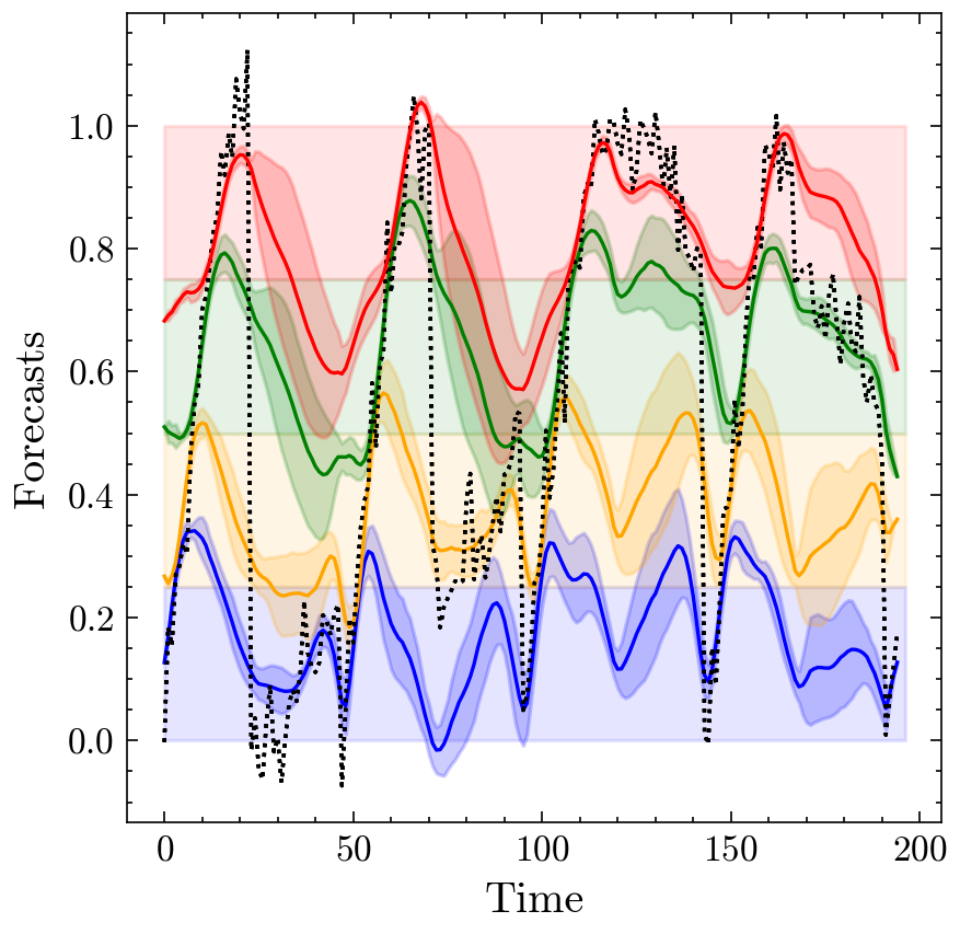
Forecasts from the iTransformer model trained using the D4-Policy, showing how it successfully captures different patterns in different value ranges.
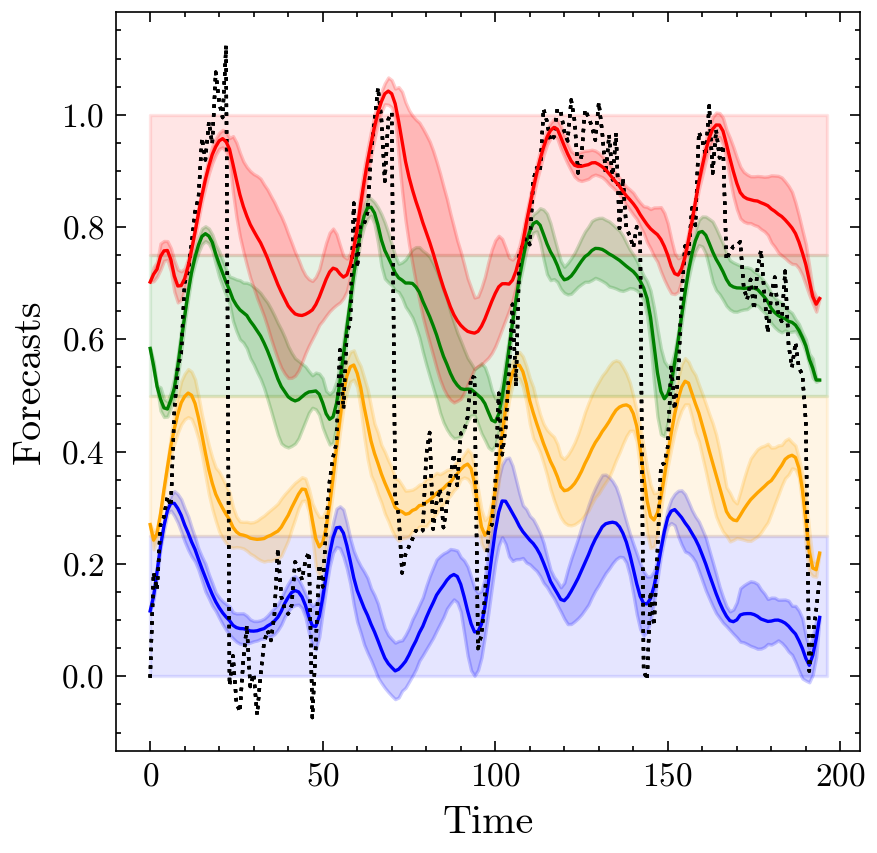
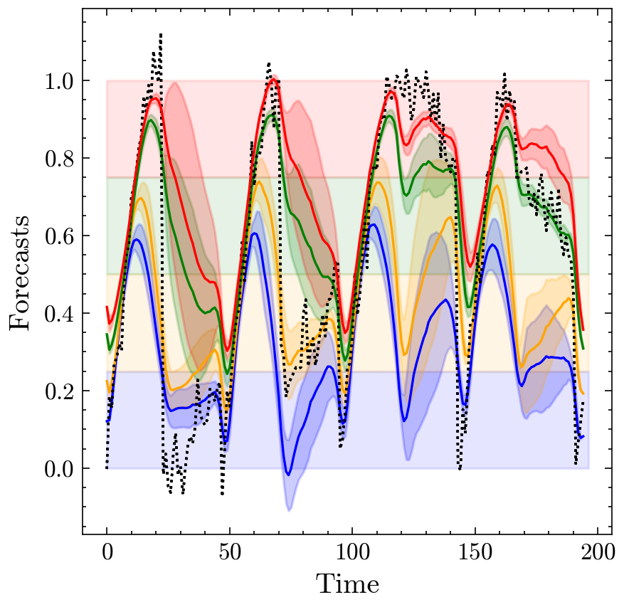
Forecasts from the iTransformer model trained using the D18-Policy, demonstrating even more fine-grained adaptation to different value ranges.
Conclusion and Future Directions
This research presents a novel training approach that transforms existing time-series forecasting models based on transformer architectures into more flexible, application-aware systems. The methodology enables a single model to adapt to various downstream tasks through adjustments during inference, rather than requiring separate models for each task.
The discrete interval training policies with interval patching (D¹ₗ-Policy and D∞ₗ-Policy) achieved the best balance of accuracy and adaptability, with improvements of up to 88% compared to the baseline approach on some datasets.
These findings have broad implications for practical applications of time-series forecasting, where different downstream tasks often have varying requirements for prediction accuracy in different value ranges.
Future research directions include:
- Scaling these models to multiple domains
- Fine-tuning publicly available time series foundation models like Timer, Moirai, and Chronos to incorporate the ability to adapt to arbitrary intervals
- Theoretical investigation into why the continuous policy (C-Policy) underperforms compared to the discrete approaches using frameworks like PAC-learning
This work provides a foundation for creating forecasting systems that better connect prediction and decision-making in various practical applications, making time-series models more useful and relevant to real-world tasks.