📌 What Are Generative Models?
Generative Models are machine learning algorithms that learn the underlying patterns or distribution of a dataset to generate new data that resembles the original.
In human terms:
They look at thousands of pictures of cats... and then start imagining their own cats.

🌟 Popular Examples of Generative Models
| Model | What It Does | Common Uses |
|---|---|---|
| GANs (Generative Adversarial Networks) | Pit 2 networks (Generator & Discriminator) against each other | Deepfakes, art generation, face synthesis |
| VAEs (Variational Autoencoders) | Probabilistic version of AEs with smooth latent space | Image reconstruction, data generation |
| Autoregressive Models | Predict next element based on previous ones | GPT, music generation |
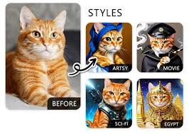
| Diffusion Models | Denoise images gradually to generate high-res outputs | DALL·E 3, Stable Diffusion |
🛣️ How Do Generative Models Learn?
Imagine you’re an artist learning how to draw cats. You spend hours going through cat books, sketching from photos, and watching cat videos on YouTube (because obviously). Over time, without memorizing each specific cat, you start to get a feel for what a “cat” is — four legs, whiskers, maybe some attitude.
Their mission:
Learn the vibe of the data so well that they can create new things that look like it.
The Typical Path:
Input Data : This is your model’s training time — a massive gallery of examples.
Think: Thousands of cat pictures (or faces, music, text). No labels needed — just raw, unfiltered examples. The model isn’t told: “This is a cat.” It just sees cats, over and over. And from that, it begins to understand patterns.Latent Representation
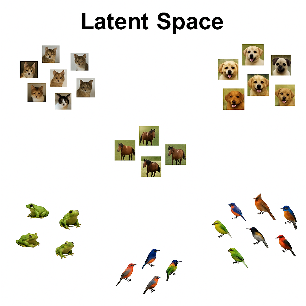
The model tries to compress all the messy, pixel-by-pixel cat data into something smaller and meaningful, kind of like the artist thinking: “Okay, I don’t remember every cat, but most cats have pointy ears, some fur texture, and this cat-ish outline... I can work with that.” In AI terms, this is the latent space — a multi-dimensional map where similar things live near each other. Imagine a universe where all cats are clustered in one corner, dogs in another, and so on.
-
Reconstruction or Generation:
Once the model has this compressed knowledge, it can do either of these:
- Reconstruct what it saw: “Can I redraw the same cat just from memory?”
- Generate something new: “Can I draw a brand new cat that no one’s ever seen, but still looks legit?” And here’s the twist — different types of models do this learning differently.
This learning can be:
Explicit (learning the actual data distribution like VAEs)
These models are like a structured student. They try to understand the actual math behind how your data is spread out, trying to learn the probability distribution. They care about making the latent space smooth, organized, and logical.
You can walk around the space, sample random points, and get meaningful results.-
Implicit (learning to fool a critic like in GANs)
These models are the street-smart artists. They don’t care about formulas — they just want their results to look good and be convincing. GANs do this through a game:- One network (the Generator) tries to create fake data
- Another (the Discriminator) tries to spot the fakes
- They improve together in a loop until the fakes are too good to tell apart.
They never explicitly learn the actual math of the data, just how to mimic it well enough to fool someone.
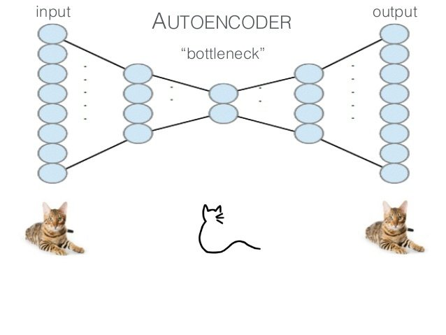
🏗️ Autoencoders Architecture (AE): Compress, Learn, Reconstruct
Let’s say we’re dealing with image data (like handwritten digits from MNIST — each image is 28x28 pixels).
Input Layer
You feed the model a raw input vector, say a flattened version of the original data (e.g., 28x28 image = 784 dims). This is just pixel intensity values (usually between 0 and 1 if normalized).
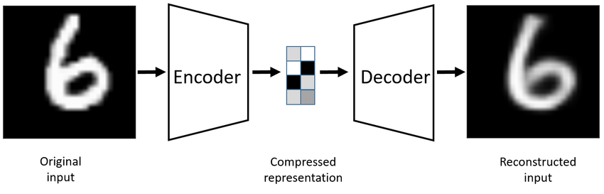
Encoder
The encoder is a neural network that compresses the input into a lower-dimensional representation — the latent vector z.
z=FuncEncoder(x)
For example, you’re squeezing 784 dimensions down to 32. Hence size of the Z vector = 2.
We want the model to learn what matters most. By forcing it to compress, the model has to filter out unimportant noise and capture the essence of the data. This is called the bottleneck. You keep only the information about the image that matters.
How can we do that?
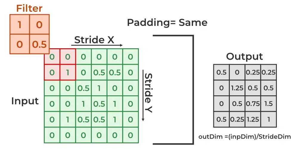
- We pass the input image (28X28) through 3 convolutional layers, one after the other.
- We use a stride of 2 (for eg), which means each layer reduces the image size by half while increasing the number of feature channels (kind of like zooming out but seeing more detail).
- So image (ColXRowXfeatureChannel) from 28X28X1 -> 14X14X32 -> 7X7X64 -> 4X4X128 sized image.
- Flatten (4 × 4 × 128) → 2048-dimensional vector
- 2048-dimensional vector Input as a Fully Connected Layer. Gives 2-Dimensional Output (Latent Vector - Z) - a compact 2D representation of your image.
Decoder
Now the decoder takes that compressed vector z and tries to rebuild the original image. It is a reverse-engineering/mirror image of the encoder.
x ′ = FuncDecoder(z)
It converts a 2D latent back to a 28*28 image.
How can we do that?
Instead of using normal convolutional layers that shrink things down, it uses transposed convolutions (or "deconvolutions") to build things back up to the original size. While a regular Conv layer with stride 2 shrinks the image, a Conv2DTranspose with stride 2 does the opposite — it doubles the size of the feature map. You can also use upsampling, which simply stretches the image to a larger size, but unlike transposed convolutions, it doesn't learn anything — it just resizes.
Here’s how the decoder does that:
- Start with the 2-dimensional latent vector (Z), and pass it through a fully connected (dense) layer to expand it into a larger vector — say, 2048 dimensions.
- Reshape that 2048-dimensional vector back into a 4 × 4 × 128 tensor, like rewinding a movie to the middle scene.
- Now we apply transposed convolutional layers (Conv2DTranspose) one after another — each with a stride of 2 — which gradually upsamples the feature maps while reducing the number of channels: 4×4×128 → 7×7×64 → 14×14×32 → 28×28×1
- The final layer outputs an image that's the same size as the input — in this case, 28×28 pixels with 1 channel (grayscale).
- Optionally, we apply a sigmoid activation at the end so all pixel values are between 0 and 1 — perfect for comparing with the original input during loss calculation!
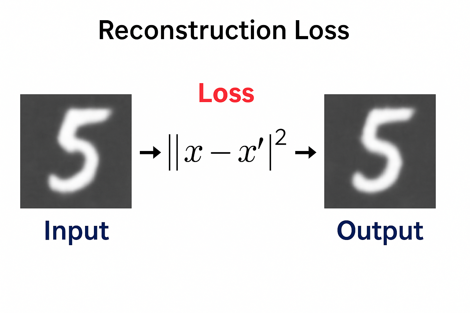
After the model reconstructs the 28*28 image, it checks the loss of the result by comparing it with the original image.
Loss Func Check
We want the input 𝑥 and the reconstruction 𝑥′ to be as close as possible.
So we minimize a loss function that measures the difference between them.
Two Common Losses:
Mean Square Error (MSE / L2 loss): It computes the square of the difference between each element in the predicted output vector and the corresponding element in the ground truth, then takes the average across all elements. This loss is particularly useful when dealing with continuous data and is known for its sensitivity to outliers.
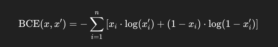
MSE Loss(J) = (1/n) * Σ(y_true - y_pred)^2Binary Cross-Entropy (BCE): used to measure the difference between two probability distributions. We use a sigmoid activation in the final layer of the decoder so that
0 < x′< 1, which makes it interpretable as a probability — a requirement for BCE to work.
The model looks at that loss and works backward( backpropagation). It figures out, layer by layer, how much each connection (weight) contributed to the mistake. Then, using an optimizer like Adam or SGD, it tweaks those weights just a little to do better next time. This process repeats again and again, and over time, the model gets good at understanding what matters in the data, like learning the essence of a handwritten “3” without being told it’s a 3.
❌ Limitations of Autoencoders

When we try to sample (pick) a random point from the latent space, we often end up with strange or meaningless outputs. That’s because some regions of the space are crowded, while others are empty, so we might accidentally pick a point from a “dead zone” where the model has never seen any training data.
Autoencoders don’t enforce any structure in the latent space. There's no rule saying, “the points should follow a neat, smooth pattern like a normal distribution.” So when we try to generate new data by sampling from the space, we don’t really know where to pick from — it's like throwing darts in the dark.
There are gaps or holes in the latent space — areas that never got used during training. The model has no clue how to decode these zones, so it often produces blurry or totally unrecognizable images.
Even points close together in space can produce wildly different outputs. For example, if (–1, –1) creates a nice image, (–1.1, –1.1) might give total noise. That’s because the model doesn’t care about making the space smooth or continuous — it's just trying to reconstruct training images.
In 2D latent spaces (for example, when visualizing MNIST), this problem isn’t too bad — everything is kind of squished together. But when we move to higher dimensions (like when generating complex stuff — faces, clothes, etc.), the gaps and discontinuities get worse. So even though more dimensions are needed to capture complex patterns, they also make the space harder to sample from safely.