This is a Plain English Papers summary of a research paper called Neural SDFs from Point Clouds: Heat Method for Accurate 3D Reconstruction. If you like these kinds of analysis, you should join AImodels.fyi or follow us on Twitter.
Introduction: A New Approach to Neural Signed Distance Fields
Neural Signed Distance Fields (SDFs) have gained popularity for representing 3D surfaces due to their flexibility and performance in applications like shape reconstruction. While many volumetric functions can represent surfaces, SDFs are preferred for additional applications such as constructive solid geometry and collision detection. They also enable the use of level set methods for solving PDEs, which have numerous applications but have only recently been explored in neural settings.
Creating an effective neural SDF requires meeting several criteria: accurate surface representation, precise non-zero level sets in a narrow band near the surface for differential computations, and the ability to be constructed directly from unoriented point clouds. Existing approaches often require approximated ground truth distances or learned priors, or they represent the zero-level set well but lack accuracy in the narrow band.
The fundamental challenge lies in solving the eikonal equation (requiring the gradient of the SDF to have unit norm), which is difficult because it has many solutions. Only the viscosity solution corresponds to the true SDF, but neural networks optimized with gradient descent may converge to non-SDF local minima.
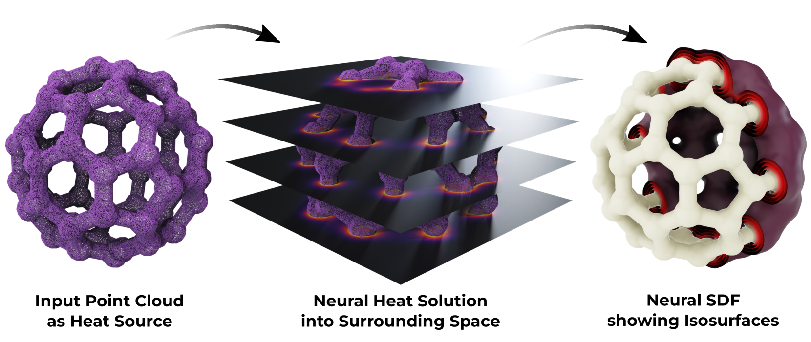
Figure 1: Visualization of the two-step process: from point cloud to heat flow to neural SDF.
This paper introduces a novel approach that replaces the eikonal equation with the heat method, a technique long used for computing distances on discrete surfaces but now adapted to the neural domain. The method defines two well-posed variational problems that can be effectively optimized with stochastic gradient descent using standard network architectures.
The heat method offers significant advantages because it avoids the challenges of the eikonal equation by solving two well-posed elliptic PDEs instead. The approach first solves for a time step of heat flow and computes the gradient of the unsigned distance function. Then, it fits the computed gradients to obtain the signed distance, considering that the input point cloud is unoriented.
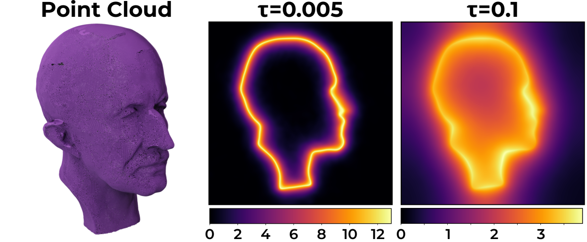
Figure 2: Visualization of the method's stages from point cloud to heat flow to SDF isosurfaces.
Compared to state-of-the-art methods, this approach (called HeatSDF) achieves a good balance between the fidelity of the zero-level set to the surface and the accuracy of the SDF in a narrow band. It works well on point clouds with non-uniform density and provides mathematical guarantees through proven existence of solutions for both steps.
The key contributions include:
- A theoretically sound variational scheme to approximate the field of level set normals and then the signed distance
- Accurate neural SDFs for spatially varying point cloud densities
- State-of-the-art surface reconstruction and accurate recovery of SDF gradients
- Application to neural PDE solving on level sets
Method: A Two-Step Approach to Computing Neural SDFs
The method considers a surface 𝒮 which is the boundary of a Lipschitz set, contained in [-1,1]³. Following the original heat method, the approach comprises two steps.
Point Clouds to Surface Normals: Step 1 of the Heat Method
In the first step, the method computes a solution u of a small time step of the heat equation with the mean surface measure as initial data. This measure is approximated via a weighted sum of point measures from the input point cloud.
The heat equation is given by:
∂ₜu - Δu = 0
Instead of using the least-squares loss for the residual, which would increase the condition number, a variational approach is employed to compute the discrete time step of heat flow. Specifically, a minimizing movements approach is used:
uᵗ := arg min₍ᵤ₎ (ℰMM(u) := ∫Ω (u-u⁰)² + τ|∇u|² dx)
Figure 3: Comparison between the gradient of a signed distance function and the normalized gradient of a heat solution.
For point clouds, the challenge is properly approximating the mean surface measure. The method normalizes the gradients of the solution to obtain an approximation of the gradient of the distance function. This works because the heat kernel is closely related to the distance function for small time steps, as explained in the neural reconstruction research.
Normals to SDF: Converting Directions to Distances
In the second step, given an approximate, unoriented normal field nᵗ, the goal is to find the SDF φ of the surface. Following Crane et al.'s approach, the method constructs an SDF approximation where φ < 0 inside the surface (with gradient pointing opposite to nᵗ) and φ > 0 outside (with gradient pointing in the same direction as nᵗ).
Figure 4: Sketch showing how the SDF gradient and heat solution gradient relate inside and outside the surface.

To achieve this, the method minimizes a normal fitting objective:
ℰₙ(φ) := ∫₍φ<0₎ |∇φ+nᵗ|² dx + ∫₍φ≥0₎ |∇φ-nᵗ|² dx
Additionally, to ensure the zero-level set coincides with the surface, a surface fitting objective is included:
ℰfit(φ) := ∫𝒮 φ² da
The sum of these two terms has at least four minima: the signed distance, the unsigned distance, and their respective negatives. To favor the SDF as the desired solution, the method introduces two sets ℬ⁻ on the inside of 𝒮 and ℬ⁺ on the outside, and defines an orientation objective:
ℰℬ(φ) := ∫ℬ⁻ χ₍φ>0₎ dx + ∫_ℬ⁺ χ₍φ<0₎ dx
This promotes φ ≤ 0 in ℬ⁻ and φ ≥ 0 in ℬ⁺. The overall objective becomes:
ℰSDF(φ) := ℰₙ(φ) + λ_fit·ℰ_fit(φ) + λℬ·ℰ_ℬ(φ)
This approach has been shown to effectively handle depth reconstruction challenges with neural SDFs.
Implementation: Technical Details
Several additional components are required for both steps of the method.
Heat Solution: Handling Point Cloud Density
To evaluate the loss functions, all examples are scaled to [-1,1]³ with a distance of at least 0.2 to the boundary of Ω. In each iteration of the descent algorithm, points are uniformly sampled from Ω and the integral is approximated by averaging the integrand's values at these points.
For the surface 𝒮 described by a point cloud (xᵢ)ᵢ₌₁,...,ₙ ⊂ ℝ³, if the cloud is uniformly distributed, the mean surface integral can be approximated by:
⨍_𝒮 u da ≈ 1/N · ∑ᵢ₌₁ᴺ u(xᵢ)
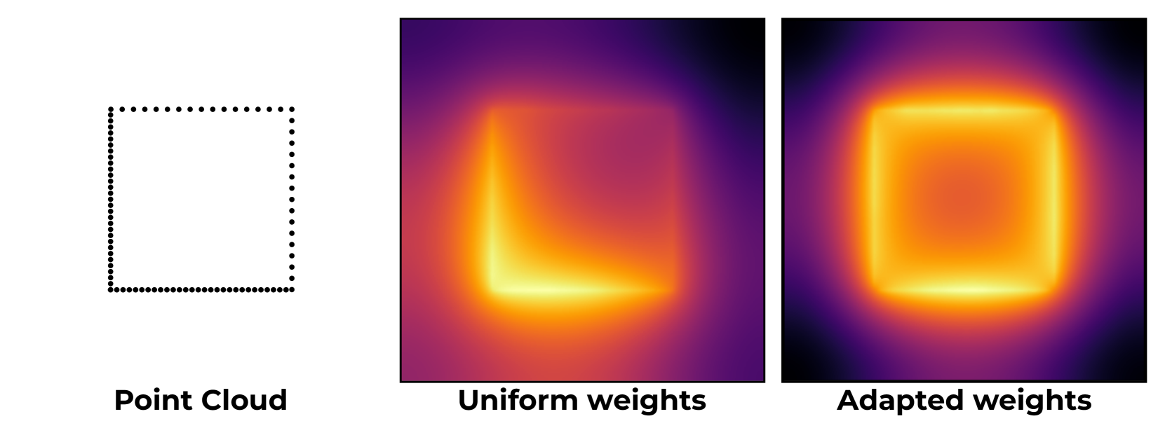
Figure 5: Comparison of heat solutions with uniform vs. adaptive weights for non-uniform point clouds.
For non-uniform distributions, a local averaging strategy is employed using adaptively weighted kernels. This approach is crucial for handling point clouds with varying density, a common challenge in learning from noisy point clouds.
Additionally, the implementation includes a "far field" heat solution to handle very small time steps while still obtaining non-zero heat throughout the domain. This is achieved by blending a far-field solution with the near-field solution based on a distance-dependent weight.
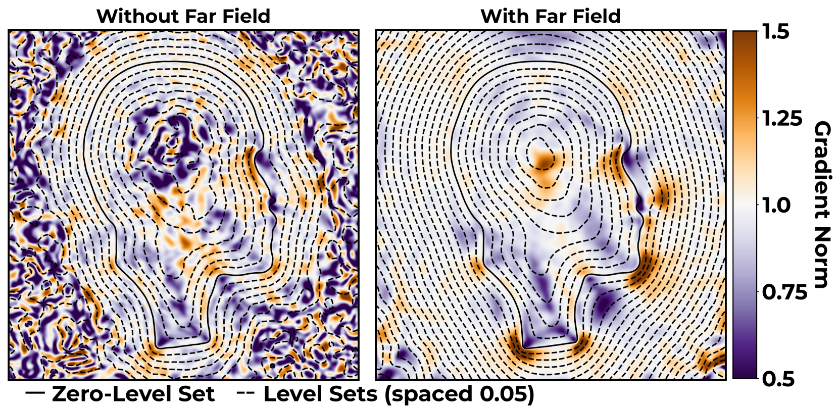
Figure 6: Comparison of level sets with and without far field blending, showing improved coverage.
SDF from Heat Solution: Determining Inside and Outside
To construct the sets ℬ⁻ (inside) and ℬ⁺ (outside), the method uses a simple and efficient algorithm that works with unoriented point clouds:
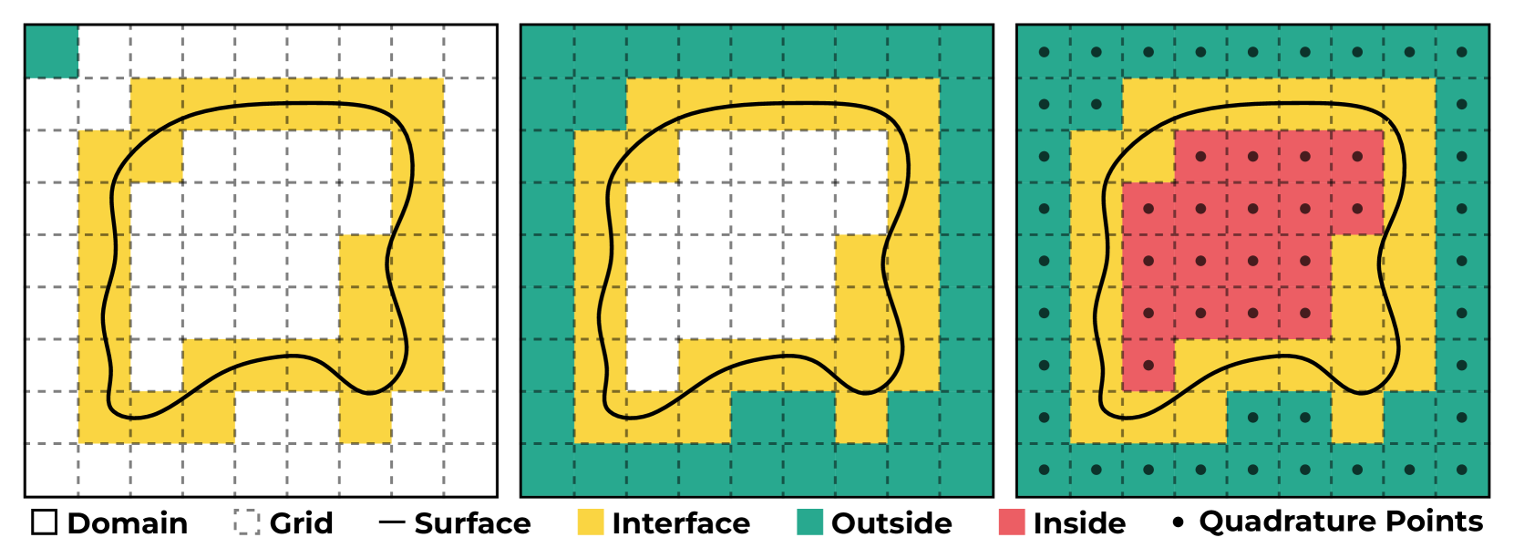
Figure 7: Illustration of the three-step algorithm for determining inside and outside regions.
- Mark all cells whose closure intersects with 𝒮 (containing points of the given point cloud) as interfacial cells.
- Starting from a cell intersecting the boundary of Ω (not marked as interfacial), successively mark each neighboring cell not yet marked as "outside."
- Mark all remaining cells as "interior."
Finally, ℬ⁺ is defined as the union of all outside cells and ℬ⁻ as the union of all inside cells. In practice, a coarse grid (e.g., 64³ points with grid size 0.0375) is sufficient.
To facilitate numerical optimization, smoothed characteristic functions are introduced to make the objective differentiable:
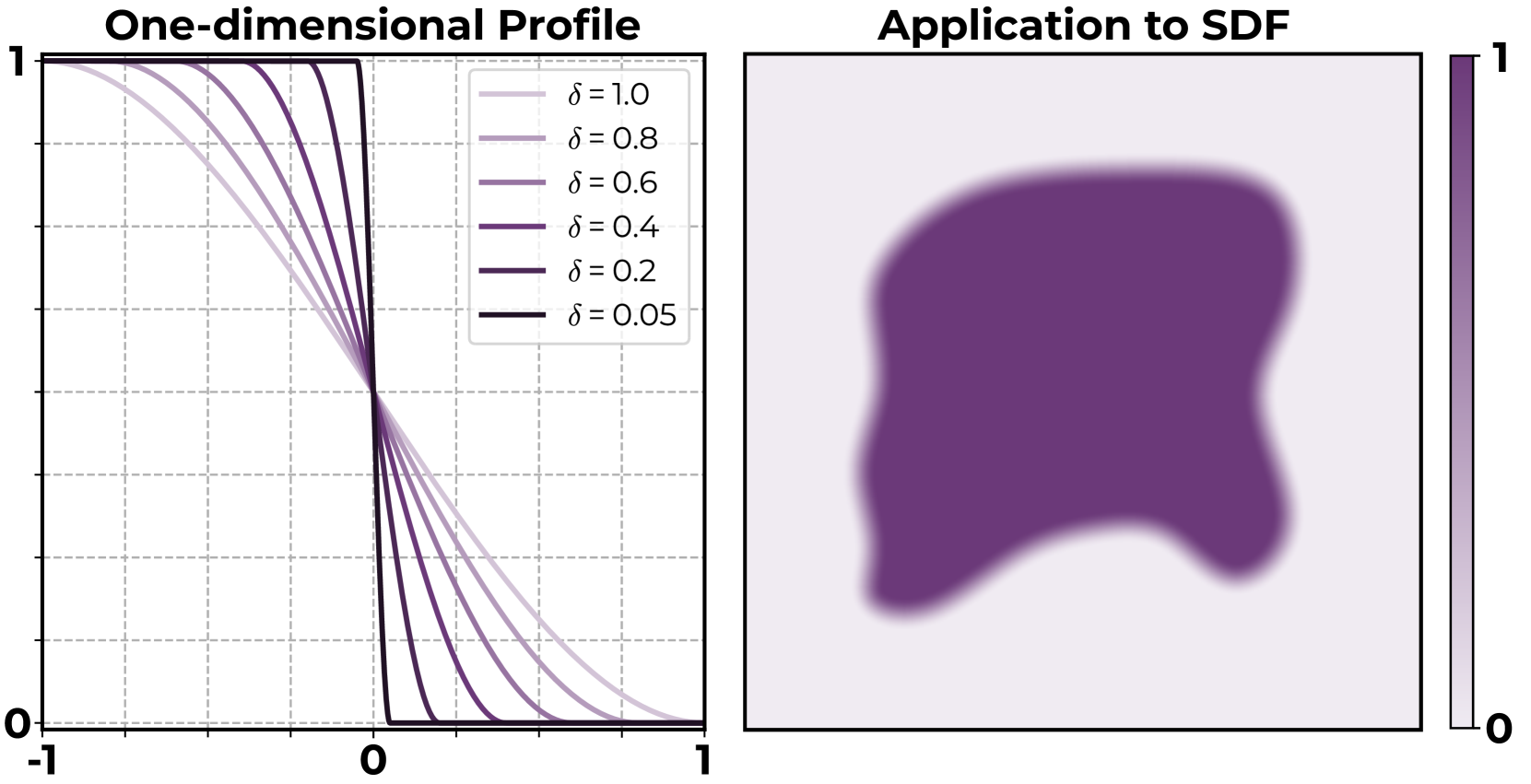
Figure 8: Visualization of the smoothed characteristic function for differentiable optimization.
Experimental Results: Validating the Heat-Based Approach
The method was implemented using the PyTorch framework. Both u and φ are represented using fully connected neural networks with four hidden layers of size 256 and sine activation functions. The Adam optimizer was used with an initial learning rate of 10⁻⁴, decreased during training. All experiments took under an hour, including both optimization steps.
Comparisons with State-of-the-Art
The method was evaluated by comparing it to other neural approaches that compute signed distance functions from point clouds, including 1-Lip (which requires oriented normals), HESS, SALD, and HotSpot.
Four evaluation metrics were used:
- E_recon^𝒮: The squared L²-error of the learned SDFs on sampled ground truth surface points.
- E_recon^n: The L¹-cosine distance between the gradients of the SDF on the zero-level set and the normals of the mesh.
- E_SDF: The L¹-error between the learned SDF and the ground truth signed distance in a narrow band.
- E_eik: The median eikonal error on a narrow band around the surface.
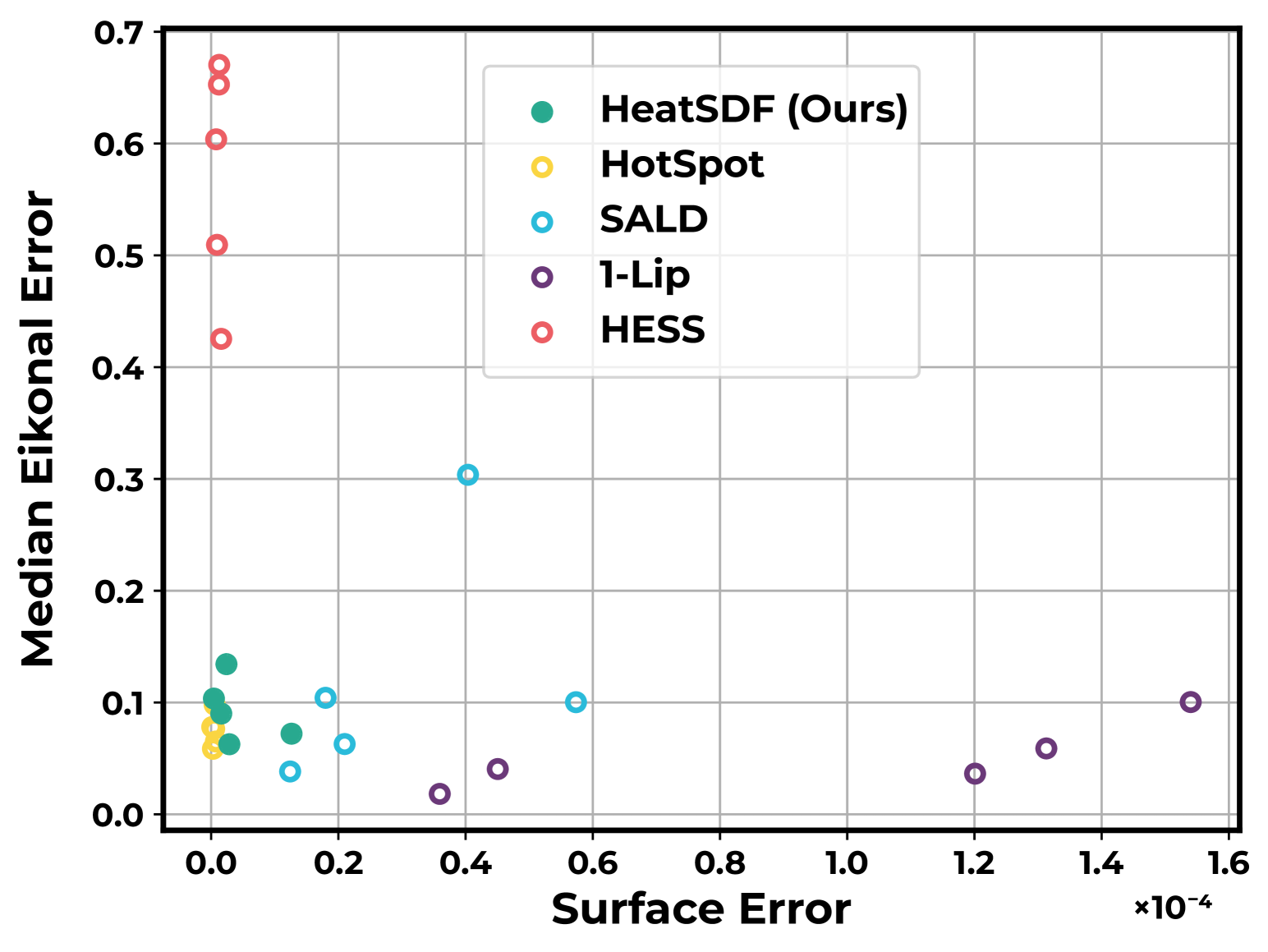
Figure 9: Comparison of surface reconstruction error vs. SDF quality measures, showing balanced performance.
The results demonstrate that the proposed method achieves a balanced trade-off between accurate surface reconstruction and good SDF approximation. In contrast, HESS produces good reconstruction results but has larger eikonal and SDF errors, while 1-Lip has low eikonal errors but loses detail in the surface reconstruction.
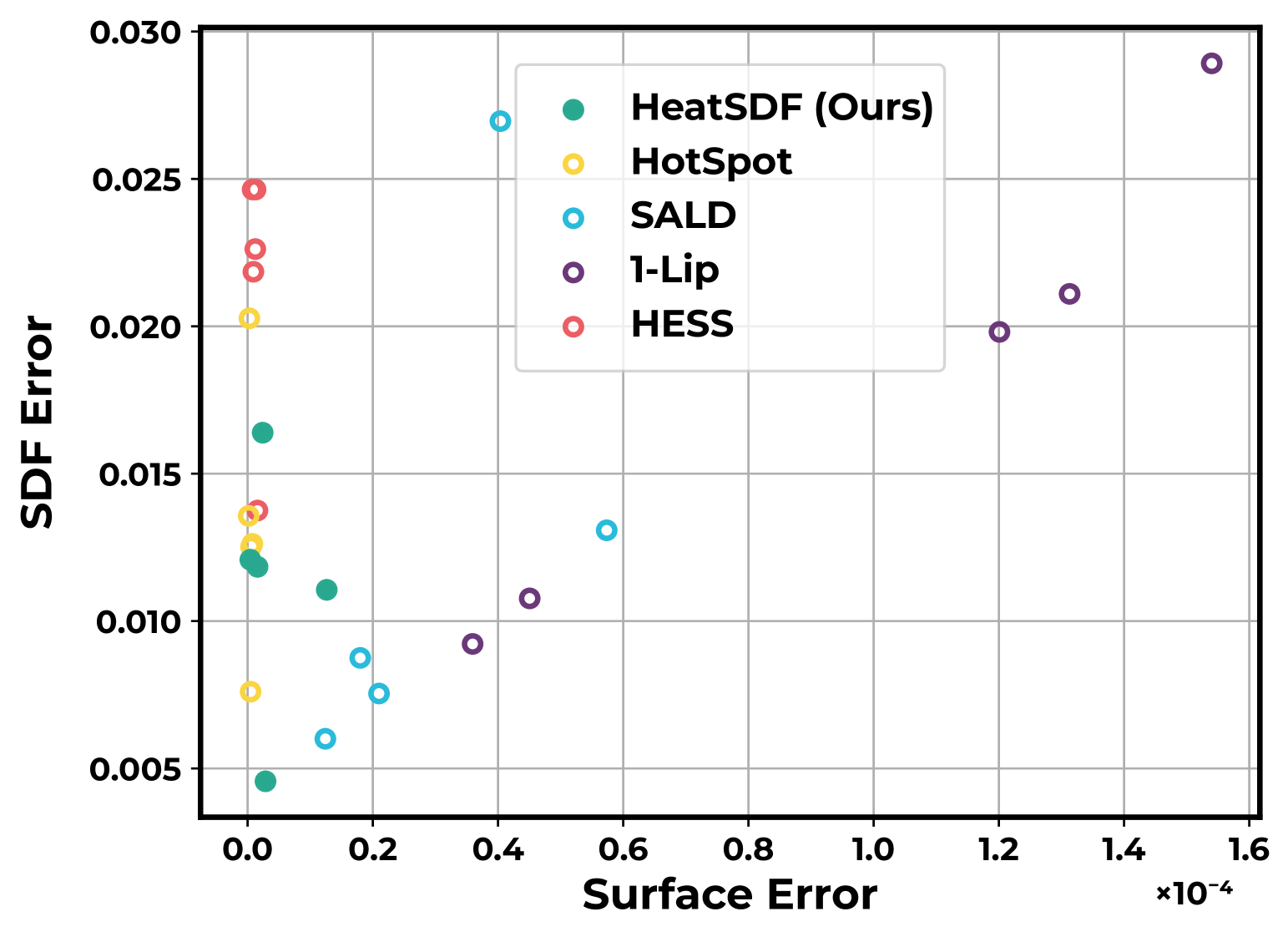
Figure 10: Visual comparison of zero-level sets and accuracy of SDF values in a narrow band near the surface.
The method also handles spatially varying point densities well, as demonstrated on a capped torus shape with dense, sparse, non-uniform, and noisy point clouds:
| Method | $\mathbf{E}_{\text {recon }}^{\text {sp }}$ | $\mathbf{E}_{\text {eik }}$ | $\mathbf{E}_{\text {recon }}^{\text {sp }}$ | $\mathbf{E}_{\text {SDF }}$ |
|---|---|---|---|---|
| SALD | $5.27 \cdot 10^{-5}$ | 0.07901 | 0.02328 | 0.00929 |
| HESS | $2.19 \cdot 10^{-7}$ | 0.73540 | 0.00004 | 0.01866 |
| 1-Lip | $1.32 \cdot 10^{-5}$ | 0.00684 | 0.00131 | 0.00339 |
| HotSpot | $1.72 \cdot 10^{-7}$ | 0.03958 | 0.00007 | 0.00699 |
| Ours | $3.85 \cdot 10^{-7}$ | 0.03529 | 0.00079 | 0.00210 |
| SALD | $3.62 \cdot 10^{-4}$ | 0.26120 | 0.08206 | 0.02397 |
| HESS | $2.21 \cdot 10^{-7}$ | 0.73540 | 0.00004 | 0.01866 |
| 1-Lip | $2.85 \cdot 10^{-5}$ | 0.00491 | 0.00191 | 0.00447 |
| HotSpot | $2.16 \cdot 10^{-6}$ | 0.03669 | 0.00044 | 0.01322 |
| Ours | $7.89 \cdot 10^{-7}$ | 0.03682 | 0.00105 | 0.00221 |
Table 1: Comparison of methods on uniform (top) and non-uniform (bottom) point clouds, showing our method maintains SDF accuracy despite varying density.
While HotSpot and SALD have difficulties with highly non-uniform point clouds (mixing inside and outside of the shape), the proposed method's SDF error only changes by a magnitude of 10⁻⁴, demonstrating its robustness to varying point densities.
Parameters and Error Metrics
The method has a weighting parameter λ_fit that controls the trade-off between surface fitting and normal alignment. Increasing λ_fit leads to better surface fitting but higher eikonal error:
| $\delta$ | $\mathbf{E}_{\text {recon }}^{\mathcal{S}}$ | $\mathbf{E}_{\text {nik }}$ |
|---|---|---|
| 0.01 | $1.312 \cdot 10^{-5}$ | 0.07020 |
| 0.0075 | $1.287 \cdot 10^{-5}$ | 0.07133 |
| 0.005 | $1.287 \cdot 10^{-5}$ | 0.07210 |
| 0.0025 | $1.248 \cdot 10^{-5}$ | 0.07381 |
| 0.001 | $1.161 \cdot 10^{-5}$ | 0.07418 |
Table 2: Impact of the smoothing parameter δ on reconstruction and eikonal errors, showing stable performance across different values.
The steepness parameter δ for the blending function shows minimal impact on performance, with the L² surface error changing only by orders of 10⁻⁶ and the eikonal error by 10⁻⁴ for δ ∈ [0.001, 0.01].
Application: Neural PDE Heat Flow on Neural Surfaces
The method can be used to solve PDEs on neural surfaces, as demonstrated with the geometric heat equation. Following previous work on level set methods, a minimizing movement scheme is formulated for this PDE application.
Given an SDF φ of a surface 𝒮, the set of parallel surfaces 𝒮c = {x ∈ Ω | φ(x) = c} is considered. The tangential gradient of a function w is ∇𝒮_φ(x) w(x) = (P∇w)(x), where P(x) = Id - n(x)⊗n(x) is the projection onto the tangent space.
Using the coarea formula and the tangential gradient, a weak formulation of the geometric heat equation ∂_t w - Δw = 0 on the level sets is obtained. This can be discretized in time using a minimizing movement formulation of a fully implicit Euler scheme.
The method was tested by computing the solution of the geometric heat equation for initial data with a Gaussian profile on the zero-level set of a neural SDF. The results show that the SDF produced by the heat-based approach is accurate enough for these challenging differential geometry tasks.
Application: Geometric Queries
The method also enables geometric operations like union and intersection of shapes:
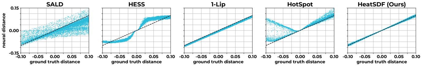
Figure 14: Visualization of a CSG union operation between two shapes using their SDFs.
For two sublevel sets [φ₁ < 0] and [φ₂ < 0], the union is [min{φ₁, φ₂} < 0] and the intersection is [max{φ₁, φ₂} < 0]. While neither min{φ₁, φ₂} nor max{φ₁, φ₂} is an SDF in general, this operation still allows for effective shape manipulation.
Limitations: Current Constraints and Future Improvements
The method has a few limitations. To ensure solving only first-order variational problems that are convex with respect to function gradients, two separate networks are trained—one for the heat diffusion time step uᵗ and one for the SDF φ.
There is also a moderate loss of detail, which is a common drawback of neural representations. Additionally, singularities such as crease lines lead to locally larger errors in the SDF. The proposed method for computing the sets ℬ± does not generalize to shapes with interior voids or disconnected internal structures, though such cases are relatively uncommon.
Conclusion and Future Work: Advancing Neural Geometry
This paper presented a novel method for computing a signed distance function from an unoriented point cloud using the heat method. Traditional approaches rely on the eikonal equation, which is inherently non-convex and can hinder convergence. The proposed method instead introduces a two-step scheme based on well-posed variational problems.
First, a time step of heat flow is computed using an approximate area measure as initial data. Then, an L² fitting of the SDF gradient is performed, using a properly reoriented and normalized gradient derived from the first step. This process results in a robust method for computing SDFs that outperforms state-of-the-art approaches in terms of the error in the signed distance function.
The method is particularly well-suited as a foundation for level set methods used to solve PDEs on surfaces. It handles non-uniform point clouds effectively and provides theoretical guarantees through proven existence of solutions for the variational problems.
Future research directions include developing narrow band adapted sampling strategies to reduce training times, optimizing network architecture, and enhancing local resolution near crease lines. Extending the method to handle more complex surface PDEs, such as thin film flow or shell deformations, remains a promising avenue for further exploration.
This work represents a significant step forward in neural implicit filtering for SDFs, combining theoretical soundness with practical performance advantages.