Co-authored with @marverickdev
Do you want to get started with machine learning, but you do not know where to start? Do you want to take advantage of the data manipulation capabilities of Python and make your own ML model locally? Well, there is a Python library designed to do just that, which is being used by startups and companies alike, and the name is Scikit-Learn!
What is Scikit-Learn, exactly?
Scikit-learn, also known as sklearn, is the primary machine learning library for Python that provides fundamental tools for both beginners and experienced developers to use for AI model training, data analysis, deep learning, and statistical modeling. It includes essential modules for classification, regression, clustering, dimensionality reduction, model selection and preprocessing. It has tools for model selection, including cross-validation methods like KFold and cross_val_score, hyperparameter search techniques such as GridSearchCV and RandomizedSearchCV, and utilizes for scoring, validation curves, and data splitting.
As is the case with most Python libraries, it is open-source and free-to-use, making it easily accessible by anyone willing to learn machine learning, and it is built upon other open-source libraries within Python, like SciPy for advanced scientific operations, NumPy for efficient numerical computations, Matplotlib for data visualization, and Cython for increased efficiency and speed, similar to that of C/C++.
Why Use Scikit-Learn?
Without libraries like scikit-learn, diving into machine learning would feel a lot like trying to bake a cake from scratch without a recipe — messy, time-consuming, and probably a little burnt. Scikit-learn hands you a ready-made toolkit packed with reliable, beginner-friendly tools for everything from classification and regression to clustering and dimensionality reduction. It’s well-documented and super popular in both classrooms and companies, like Spotify, AWS, J.P Morgan, and Evernote, meaning there’s always someone who’s faced the same problem you’re tackling. And because it’s actively maintained, you’re not stuck using outdated methods — you get access to the latest techniques without the hassle.
From a developer’s point of view, scikit-learn is like having a set of interchangeable LEGO bricks. Its consistent, clean interface means you don’t have to memorize a million different function names for different algorithms. Whether you’re using a decision tree or a support vector machine, you’ll be calling familiar functions like fit(), predict(), and score(). This makes experimenting way smoother, leaving developers free to focus on building smarter models, rather than wrestling with complicated code. Plus, its active community means plenty of tutorials, updates, and fixes are always within reach.
Scikit-Learn vs. TensorFlow vs. Pytorch
Scikit-Learn, TensorFlow, and PyTorch are three of the most widely used libraries in machine learning and deep learning, each serving different purposes and catering to distinct workflows.
Scikit-Learn is the go-to library for classical machine learning tasks, offering a simple and consistent API for algorithms like linear regression, support vector machines (SVMs), and random forests. It excels in handling small-to-medium-sized structured datasets (e.g., CSV files) and is built on NumPy and SciPy, making it efficient for CPU-based computations. However, it lacks native GPU support and is not designed for deep learning—though it does include a basic multi-layer perceptron (MLP) for simple neural networks. Scikit-Learn is ideal for tasks like customer segmentation, fraud detection, and traditional predictive modeling where deep learning is unnecessary.
TensorFlow, developed by Google, is a powerful framework for deep learning, particularly suited for large-scale neural network training and deployment. Its high-level Keras API simplifies model building, while its low-level operations allow for fine-grained control. TensorFlow supports distributed training, making it a strong choice for production environments, and it integrates well with mobile (LiteRT) and web deployment (TensorFlow.js). It is widely used in industry for applications like image recognition, natural language processing (NLP), and recommender systems. While it has a steeper learning curve than Scikit-Learn, its robustness and scalability make it a favorite for production-grade deep learning.
PyTorch, developed by Meta (Facebook), is the preferred framework for research and rapid prototyping in deep learning. Its dynamic computation graph (eager execution) allows for more intuitive debugging and flexibility, making it popular in academia and cutting-edge research. PyTorch’s Pythonic design and strong GPU acceleration (via CUDA) enable quick experimentation with novel architectures like transformers, generative adversarial networks (GANs), and reinforcement learning models. While historically lagging behind TensorFlow in deployment tools, PyTorch has improved significantly with TorchScript and ONNX support, narrowing the gap. Researchers and startups often favor PyTorch for its ease of use and dynamic nature.
Choosing the Right Tool
- Use Scikit-Learn for classical ML tasks where deep learning is overkill.
- Use TensorFlow for scalable deep learning in production, especially when deployment is a priority.
- Use PyTorch for research, experimentation, and when flexibility in model design is crucial.
Getting Started with Scikit-Learn
Creating a Virtual Environment (Optional)
Before we can go ahead with the installation, it is recommended to create a virtual environment for Python so that the installation is isolated to the project. To do so, type this command in your preferred IDE’s terminal (We will be using VS Code for this guide):
python -m venv .venvKeep in mind that this is optional when you are to get started in Python and Scikit-Learn, but this is a precaution to prevent any unexpected errors in your other Python projects.
Installation
To install Scikit-Learn into your project, enter this command in the terminal:
python -m pip install scikit-learnwhen you are using VS Code, this would ensure that the packages install in the selected Python environment.
Importing Scikit-Learn Modules
You can import different parts of Scikit-Learn depending on what you need.
Here’s an example:
from sklearn.datasets import load_iris
from sklearn.model_selection import train_test_split
from sklearn.linear_model import LogisticRegression
from sklearn.metrics import accuracy_score
Basic Workflow in Scikit-Learn
📌Import Necessary Modules
Use modules that are important for your project/use case (e.g. Logistic Regression)
from sklearn.datasets import load_iris
from sklearn.model_selection import train_test_split
from sklearn.linear_model import LogisticRegression
from sklearn.metrics import accuracy_score
📌Load and Prepare Data
Import the dataset for training
# Example with built-in dataset
from sklearn.datasets import load_iris
data = load_iris()
X = data.data  # Features
y = data.target  # Target variable
📌Split Data into Training and Test Sets
Set the variables for data splitting, which splits the dataset into subsets used for data training and testing
X_train, X_test, y_train, y_test = train_test_split(
    X, y, test_size=0.2, random_state=42
)
📌Preprocess the Data
Preprocessing cleans the dataset such that it can be read by the model and make it suitable for training and testing
scaler = StandardScaler()
X_train = scaler.fit_transform(X_train)
X_test = scaler.transform(X_test)  # Note: Only transform the test set
📌Choose and Train a Model
Choose the model that you imported in the first step
model = LogisticRegression(max_iter=200)
model.fit(X_train, y_train)
📌Make Predictions (if learning is supervised)
Supervised learning trains the model to make connections or predictions based on the dataset the model is being trained on
y_pred = model.predict(X_test)📌Evaluate the Model
Tests the accuracy of the model
accuracy = accuracy_score(y_test, y_pred)
print(f"Accuracy: {accuracy:.2f}")
How to use Scikit-Learn
Scikit-learn follows a consistent API pattern across all algorithms:
- Import the appropriate model
- Instantiate the model with parameters
- Fit the model to your data
- Predict or evaluate with new data
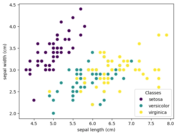
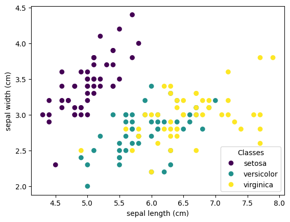
Example 1: Classification (Iris Dataset)
Separates the data based on the type of irises and their petal and sepal length & width
# Importing required libraries
from sklearn.datasets import load_iris
from sklearn.model_selection import train_test_split
from sklearn.neighbors import KNeighborsClassifier
from sklearn.metrics import accuracy_score

# 1. Load dataset
iris = load_iris()
X, y = iris.data, iris.target

# 2. Split data into training and test sets
X_train, X_test, y_train, y_test = train_test_split(
    X, y,
    test_size=0.2,
    random_state=42
)

# 3. Initialize and train KNN classifier
knn = KNeighborsClassifier(n_neighbors=3)
knn.fit(X_train, y_train)

# 4. Make predictions and evaluate model
predictions = knn.predict(X_test)
print(f"Accuracy: {accuracy_score(y_test, predictions):.2f}")
Output (from matplotlib.pyplot)
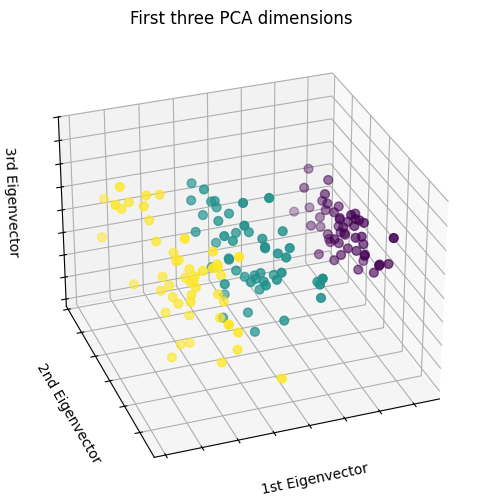
Output (from Principal Component Analysis [PCA])
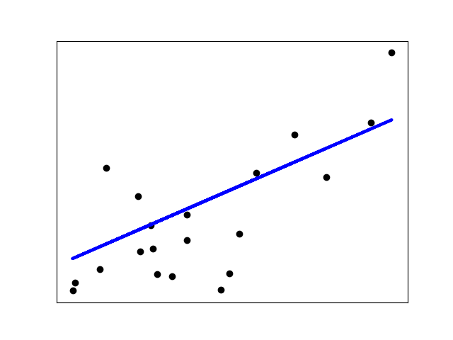
Example 2: Regression (Diabetes)
Illustrates the pattern of diabetes patients through regression, which estimates the relationships between the various patient features and the presence of diabetes
# Importing required libraries
import matplotlib.pyplot as plt
import numpy as np
from sklearn import datasets, linear_model
from sklearn.metrics import mean_squared_error, r2_score

# 1. Load and prepare dataset
diabetes_X, diabetes_y = datasets.load_diabetes(return_X_y=True)
diabetes_X = diabetes_X[:, np.newaxis, 2]  # Use only one feature

# 2. Split data into training and test sets
diabetes_X_train = diabetes_X[:-20]
diabetes_X_test = diabetes_X[-20:]
diabetes_y_train = diabetes_y[:-20]
diabetes_y_test = diabetes_y[-20:]

# 3. Create and train linear regression model
regr = linear_model.LinearRegression()
regr.fit(diabetes_X_train, diabetes_y_train)

# 4. Make predictions and evaluate model
diabetes_y_pred = regr.predict(diabetes_X_test)
print("Coefficients: \n", regr.coef_)
print("Mean squared error: %.2f" % mean_squared_error(diabetes_y_test, diabetes_y_pred))
print("Coefficient of determination: %.2f" % r2_score(diabetes_y_test, diabetes_y_pred))

# 5. Visualize results
plt.scatter(diabetes_X_test, diabetes_y_test, color="black")
plt.plot(diabetes_X_test, diabetes_y_pred, color="blue", linewidth=3)
plt.xticks(())
plt.yticks(())
plt.show()
Output (from matplotlib)
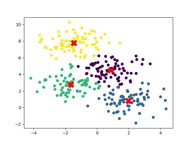
Example 3: Clustering (K-Means)
Groups similar data into one area (clusters) and pinpoint the center of each area (means)
# Importing required libraries
from sklearn.cluster import KMeans
from sklearn.datasets import make_blobs
import matplotlib.pyplot as plt

# 1. Create synthetic data
X, y = make_blobs(n_samples=300, centers=4, random_state=42)

# 2. Create and fit model
kmeans = KMeans(n_clusters=4)
kmeans.fit(X)

# 3. Get cluster assignments
labels = kmeans.labels_

# 4. Visualization
plt.scatter(X[:, 0], X[:, 1], c=labels, cmap='viridis')
plt.scatter(kmeans.cluster_centers_[:, 0], kmeans.cluster_centers_[:, 1], s=200, c='red', marker='X')
plt.show()
Output (from matplotlib)
Tips for Effective Use
- Always split your data into training and test sets
- Preprocess your data appropriately (scaling, encoding, etc.)
- Start with simple models before trying complex ones
- Use cross-validation to evaluate model performance
- Explore the extensive documentation for each algorithm's parameters
Other Examples of Models in Scikit-Learn
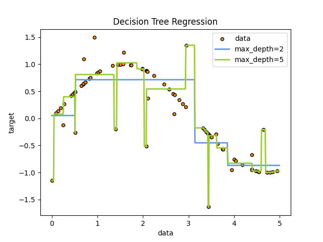
1️⃣Decision Tree
What it Does: It makes predictions by learning simple rules from data.
When to use: When you need an interpretable model (but can overfit).
# Import required libraries
import numpy as np
from sklearn.tree import DecisionTreeRegressor
import matplotlib.pyplot as plt

# 1. Generate synthetic data (sine wave with noise)
rng = np.random.RandomState(1)
X = np.sort(5 * rng.rand(80, 1), axis=0)
y = np.sin(X).ravel()
y[::5] += 3 * (0.5 - rng.rand(16))  # Add noise to every 5th point

# 2. Initialize and train models
regr_shallow = DecisionTreeRegressor(max_depth=2)  # Simple model
regr_deep = DecisionTreeRegressor(max_depth=5)     # Complex model
regr_shallow.fit(X, y)
regr_deep.fit(X, y)

# 3. Create test data and predictions
X_test = np.arange(0.0, 5.0, 0.01)[:, np.newaxis]
y_shallow = regr_shallow.predict(X_test)
y_deep = regr_deep.predict(X_test)

# 4. Visualize results
plt.figure(figsize=(10, 6))
plt.scatter(X, y, s=20, edgecolor="black", c="darkorange", label="Data")
plt.plot(X_test, y_shallow, color="cornflowerblue", label="max_depth=2", linewidth=2)
plt.plot(X_test, y_deep, color="yellowgreen", label="max_depth=5", linewidth=2)
plt.xlabel("X")
plt.ylabel("y")
plt.title("Decision Tree Regression: Effect of Tree Depth")
plt.legend()
plt.show()
Output (from matplotlib)
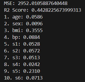
2️⃣Random Forest
What it does: Ensemble of decision trees (more accurate, less overfitting).
When to use:When you want a robust, "just works" model.
# Import required libraries
from sklearn.datasets import load_diabetes
from sklearn.ensemble import RandomForestRegressor
from sklearn.metrics import mean_squared_error, r2_score
from sklearn.model_selection import train_test_split

# 1. Load the diabetes dataset
data = load_diabetes()
X = data.data  # Features (medical measurements)
y = data.target  # Target variable (disease progression score)

# 2. Split data into training and test sets (80% train, 20% test)
X_train, X_test, y_train, y_test = train_test_split(
    X, y, test_size=0.2, random_state=42
)

# 3. Train a Random Forest Regressor
model = RandomForestRegressor(n_estimators=100, random_state=42)
model.fit(X_train, y_train)

# 4. Predict on the test set and evaluate performance
y_pred = model.predict(X_test)
print("MSE:", mean_squared_error(y_test, y_pred))  # Lower is better
print("R² Score:", r2_score(y_test, y_pred))       # Closer to 1 is better

# 5. Display feature importances (which variables matter most?)
importances = model.feature_importances_
for i, (feature, importance) in enumerate(zip(data.feature_names, importances)):
    print(f"{i+1}. {feature}: {importance:.4f}")
Output (from terminal)
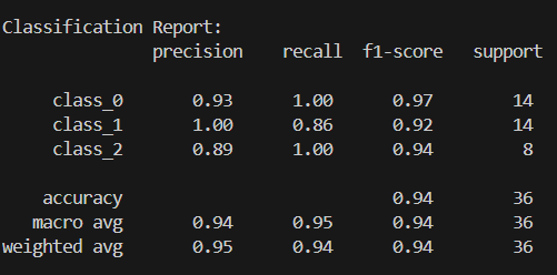
3️⃣k-Nearest Neighbors (k-NN)
What it does: Predicts based on the closest training examples (no training needed).
When to use: For small datasets or when local patterns matter.
# Import required libraries
from sklearn.datasets import load_wine
from sklearn.neighbors import KNeighborsClassifier
from sklearn.model_selection import train_test_split
from sklearn.preprocessing import StandardScaler
from sklearn.metrics import accuracy_score, classification_report

# 1. Load the Wine dataset
wine = load_wine()
X = wine.data  # Features (chemical properties)
y = wine.target  # Target variable (wine class: 0, 1, or 2)

# 2. Split data into training and test sets (80% train, 20% test)
X_train, X_test, y_train, y_test = train_test_split(
    X, y, test_size=0.2, random_state=42
)

# 3. Standardize features (critical for distance-based models like KNN)
scaler = StandardScaler()
X_train = scaler.fit_transform(X_train)  # Fit on train, transform train
X_test = scaler.transform(X_test)        # Transform test (no fitting)

# 4. Train a KNN classifier with 3 neighbors
model = KNeighborsClassifier(n_neighbors=3)
model.fit(X_train, y_train)

# 5. Predict and evaluate performance
y_pred = model.predict(X_test)
print("Accuracy:", accuracy_score(y_test, y_pred))
print("\nClassification Report:\n", classification_report(y_test, y_pred))
Output (from terminal)
Conclusion
As you can see, Scikit-Learn has many uses and applications that are critical for our daily lives, many of which we are not aware of. From research and predictive analytics to natural language processing and recommendation algorithms, all can be easily done with the help of this Python library. So, if you are looking for a great starting point in the realm of machine learning, consider going deep into Scikit-Learn for your first ML project.
If you want to learn more about Scikit-Learn, you can refer to the official user guide for further details.
References / Materials:
https://www.ibm.com/think/topics/scikit-learn#:~:text=Scikit-learn%2C%20or%20sklearn%2C,modeling%20with%20a%20consistent%20interface.
https://scikit-learn.org/stable/testimonials/testimonials.html
https://www.analyticsvidhya.com/blog/2021/07/15-most-important-features-of-scikit-learn/
https://scikit-learn.org/1.5/auto_examples/linear_model/plot_ols.html