Hey friends! 👋
Today, we’re diving into something really cool: predicting stock prices using an LSTM (Long Short-Term Memory) neural network 🧠!. If you’re curious about machine learning, stock market forecasting, or just love tinkering with data, this post is for you! Let’s break down the process in a friendly, approachable way, based on a Jupyter Notebook I worked on (Notebook Link).
What’s This All About?
The goal of this project was to predict the future stock prices of Microsoft (ticker: MSFT) using historical data and an LSTM model. LSTMs are a type of neural network particularly great for handling time-series data, like stock prices, because they can "remember" patterns over long periods. Think of them as a super-smart friend who can spot trends in data and make educated guesses about what’s coming next.
In my notebook, I used Python libraries like yfinance to grab stock data, pandas and numpy for data wrangling, and pytorch to build the LSTM model. The result? A model that forecasts stock prices and visualizes how well it performs. Let’s walk through the key steps and sprinkle in some insights along the way!
📚 Step 1: Gathering Our Data
First things first, we need data to work with. I used the yfinance library to download Microsoft’s (MSFT) daily stock data from January 1, 2017, up to about a month ago (March 25, 2025, in my case). Here’s a peek at the code I used:
import numpy as np
import pandas as pd
import matplotlib.pyplot as plt
import seaborn as sns

import yfinance as yf
import datetime as dt

from sklearn.preprocessing import StandardScaler
Next, we define the start and end dates for our dataset:
start_date = dt.datetime(2017,1,1)
end_date = dt.datetime.now() - dt.timedelta(days=30)
We then load the historical data using a custom function load_ticker_data:
def load_ticker_data(ticker_symbol, start_date="2020-01-01", end_date=None, interval="1d"):
"""
Load historical data for a given ticker from Yahoo Finance.
Args:
ticker_symbol (str): The stock ticker symbol (e.g., 'AAPL').
start_date (str): The start date for the historical data (YYYY-MM-DD).
end_date (str): The end date for the data. If None, fetches up to today.
interval (str): Data interval ('1d', '1wk', '1mo', etc.).
Returns:
pandas.DataFrame: Historical price data for the ticker.
"""
ticker = yf.Ticker(ticker_symbol)
data = ticker.history(start=start_date, end=end_date, interval=interval)
return data
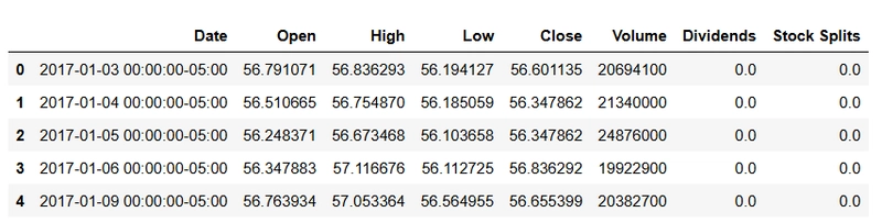
data = load_ticker_data('MSFT', start_date=start_date, end_date=end_date, interval='1d')This gave me a neat pandas DataFrame with columns like Date, Open, High, Low, Close, Volume. For this project, I focused on the Close price, as it’s a common choice for stock price prediction.
Fun Fact: The data included over 2,000 trading days, giving us plenty of historical patterns to feed into the LSTM model!
🛠 Step 2: Exploring the Data
Let's take a look at the first few rows of our dataset:
data.head()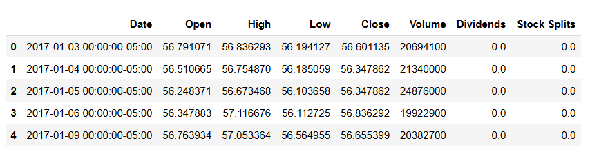
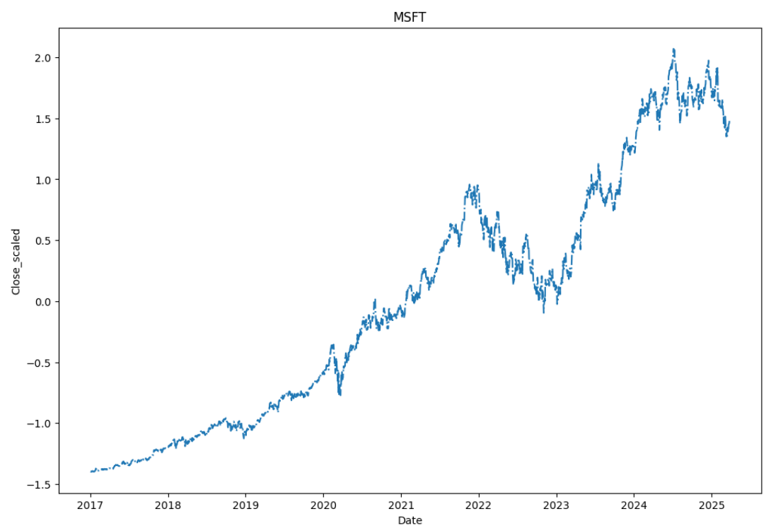
We also plotted the closing prices to see how the stock moved over time 📈.
plt.figure(figsize=(12,8))
sns.lineplot(data=data,x='Date',y='Close',linestyle='--')
plt.title("MSFT")
plt.show()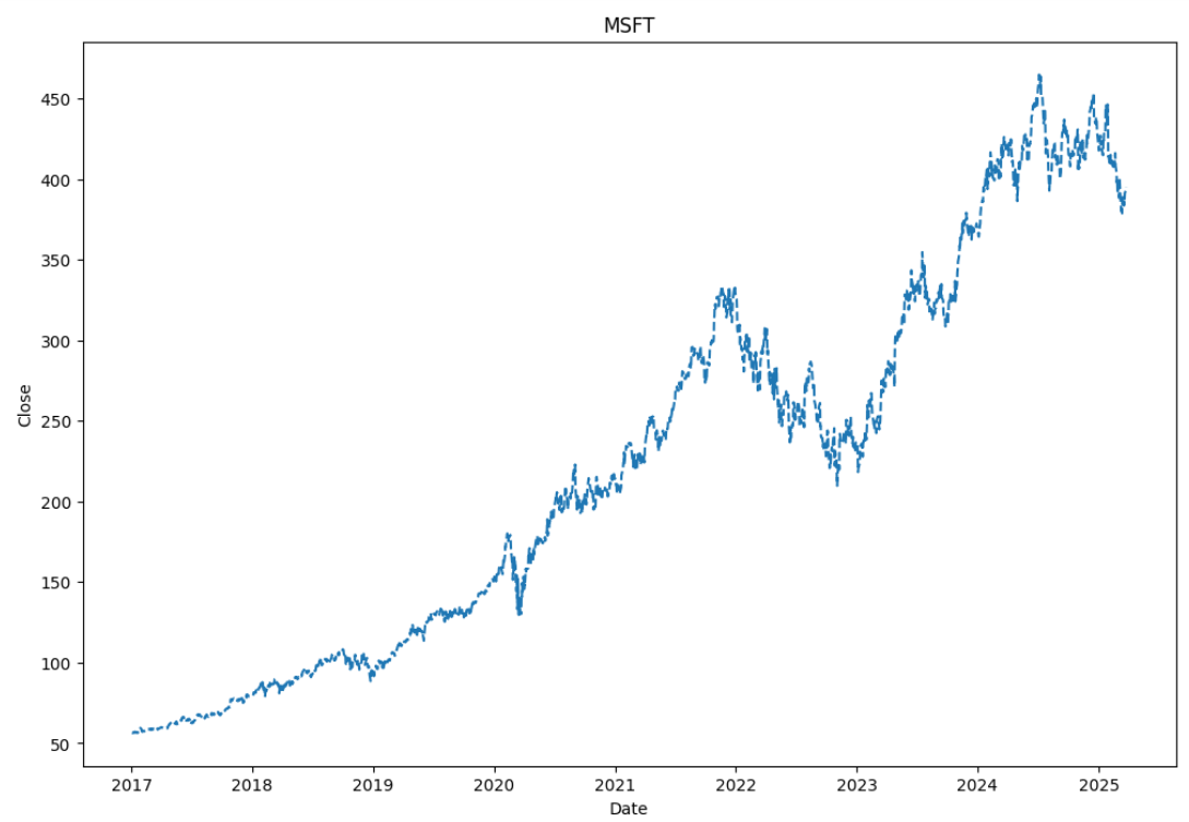
🧹 Step 3: Preparing the Data for the Neural Network
Before feeding data to our LSTM model, we need to clean and normalize it. We:
- Scaled the closing prices using StandardScaler (because neural networks love numbers between -1 and 1).
- Created sequences of 60 days to predict the next day’s price (like teaching the model to recognize patterns).
sd_scaler = StandardScaler()

data[['Close_scaled']] = sd_scaler.fit_transform(data[['Close']])
Here is the scaled data chart
prediction_days=60
#x-train : 0-59 days, y_train : 1 day (60th day)

x_train, y_train = [], []

for x in range(prediction_days, len(scaled_close_prices)):
    x_train.append(scaled_close_prices[x-prediction_days:x,0])
    y_train.append(scaled_close_prices[x,0])
x_train = np.array(x_train)
y_train = np.array(y_train)
x_train_r = x_train.reshape(x_train.shape[0],x_train.shape[1],1)
print(x_train_r.shape, y_train.shape)
(2008, 60, 1) (2008,)
Now the data is ready for the model! 🔥
🏗 Step 4: Building the LSTM Model
We built a 3-layer LSTM model with a bit of dropout to prevent overfitting:
import torch
import torch.nn as nn
import torch.nn.functional as F
from torchinfo import summary
import torch.optim as optim
from torch.utils.data import DataLoader, TensorDataset
import numpy as np
from tqdm import tqdm

device = torch.device("cuda" if torch.cuda.is_available() else "cpu")

class LSTMModel(nn.Module):
    def __init__(self, input_size=1, hidden_size=96, dropout_rates=[0.3, 0.2, 0.1]):
        super(LSTMModel, self).__init__()
        self.hidden_size= hidden_size

        self.lstm1 = nn.LSTM(input_size=input_size, hidden_size=hidden_size,
                             num_layers=1, batch_first=True)
        self.dropout1 = nn.Dropout(dropout_rates[0])

        self.lstm2 = nn.LSTM(input_size=hidden_size, hidden_size=hidden_size,
                             num_layers=1, batch_first=True)
        self.dropout2 = nn.Dropout(dropout_rates[1])

        self.lstm3 = nn.LSTM(input_size=hidden_size, hidden_size=hidden_size,
                             num_layers=1, batch_first=True)
        self.dropout3 = nn.Dropout(dropout_rates[2])


        self.fc = nn.Linear(hidden_size, 1)

    def forward(self, x):
        batch_size = x.size(0)

        h0 = torch.zeros(1, batch_size, self.hidden_size).to(x.device)
        c0 = torch.zeros(1, batch_size, self.hidden_size).to(x.device)

        out, _ = self.lstm1(x, (h0, c0))
        out = self.dropout1(out)

        out, _ = self.lstm2(out)
        out = self.dropout2(out)

        out, _ = self.lstm3(out)
        out = self.dropout3(out[:, -1, :])

        out = self.fc(out)

        return out

# Initialize Clean Model
model = LSTMModel(hidden_size=96, dropout_rates=[0.3,0.2,0.1])

# Assume input shape is (batch_size=32, sequence_length=60, features=1)
summary(model, input_size=(32, 60, 1))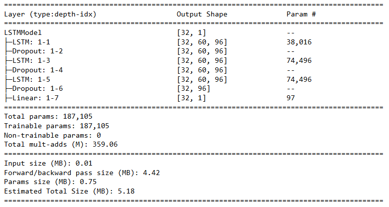
🏋️ Step 5: Training the Model
# ==== CUSTOM DATA LOADING ====
def get_dataloaders_from_numpy(x_train_r, y_train, batch_size=64):
    x_tensor = torch.tensor(x_train_r, dtype=torch.float32)  # (n, 60 days, 1)
    y_tensor = torch.tensor(y_train, dtype=torch.float32).view(-1, 1)  # (n, 1)

    dataset = TensorDataset(x_tensor, y_tensor)
    train_loader = DataLoader(dataset, batch_size=batch_size, shuffle=True)
    return train_loader
# ==== TRAINING LOOP ====
def train(model, train_loader, epochs=20, lr=0.001, device='cuda'):
    model.to(device)
    criterion = nn.MSELoss()
    optimizer = optim.Adam(model.parameters(), lr=lr)
    last_loss = 0.0
    for epoch in range(epochs):
        model.train()
        running_loss = 0.0
        for x_batch, y_batch in tqdm(train_loader, desc=f"Epoch {epoch+1}/{epochs}, Loss {last_loss}"):
            x_batch, y_batch = x_batch.to(device), y_batch.to(device)

            optimizer.zero_grad()
            outputs = model(x_batch)
            loss = criterion(outputs, y_batch)
            loss.backward()
            optimizer.step()

            running_loss += loss.item()

        avg_loss = running_loss / len(train_loader)
        last_loss = avg_loss

train_loader = get_dataloaders_from_numpy(x_train_r, y_train, batch_size=32)
train(model, train_loader, epochs=10, lr=0.0001, device=device)
We trained the model for 10 epochs (iterations) with:
- Learning rate = 0.0001 (slow and steady wins the race 🐢).
- Batch size = 32 (small chunks for better learning).
🔮 Step 6: Making Predictions!
Now for the magic trick ✨: forecasting future prices!
We used the last 30 days to predict the next 30 days 📆. We also added a tiny bit of randomness (temperature) to mimic the uncertainty of real stock markets 🎲.
def model_infer(model, input_starting_60_days, prediction_length=10, temperature=0.001, scaler=None, device='cpu'):
    model.eval()
    last_60_data = input_starting_60_days.copy()
    # add last day in given data
    predictions = [sd_scaler.inverse_transform(last_60_data[-1])[0]]

    for _ in range(prediction_length-1):
        # Prepare input tensor: shape (1, 60, 1)
        input_tensor = torch.tensor(last_60_data, dtype=torch.float32).unsqueeze(0).to(device)

        with torch.no_grad():
            output = model(input_tensor)  # shape (1, 1)
            output = output.cpu().numpy()  # convert to NumPy
            output += np.random.randn(1) * temperature  # add temperature to LSTM (mimic market uncertainity)

        predictions.append(sd_scaler.inverse_transform(output)[0][0])  # append scalar value
        last_60_data = np.vstack((last_60_data, output))[-60:]  # slide window

    return predictions

test_duration = 30
test_start =  dt.datetime.now() - dt.timedelta(days=test_duration)
test_end = dt.datetime.now()

test_data = load_ticker_data(ticker, start_date=test_start , end_date=test_end , interval='1d')
test_data = test_data.reset_index()

# get last
input_to_lstm_duration = 30
last_days_in_training = data.iloc[-input_to_lstm_duration:].copy()
scaled_close_prices_test = sd_scaler.transform(last_days_in_training['Close'].values.reshape(-1,1))

# Prepare starting sequence
input_sequence = scaled_close_prices_test

# Inference
predictions = model_infer(model, input_sequence, prediction_length=test_duration, temperature=0.01, device=device)

predictions_ = np.array(predictions).squeeze()
predicted_dates = pd.date_range(start=data['Date'].iloc[-1], periods=len(predictions))
prediction_df = pd.DataFrame({'Date': predicted_dates, 'Predicted Close': predictions})

plt.figure(figsize=(16,9))

t_range = 2000
plt.title(f"{ticker}")
sns.lineplot(x=data.iloc[t_range:].Date,y= data.iloc[t_range:].Close,linestyle='-',color='gray', label='History (Train) Data')

sns.lineplot(x=test_data.Date,y= test_data.Close,linestyle=':',color='green', label='Forecasted (Test) Data')

sns.lineplot(x=prediction_df['Date'], y=prediction_df['Predicted Close'],linestyle='-.',color='blue', label='Neural Prediction')
plt.show()
And of course, we visualized it beautifully:
- Gray line: Historical (training) data
- Green dots: Real test data (past month)
- Blue dashed line: Model's predicted future 🎯
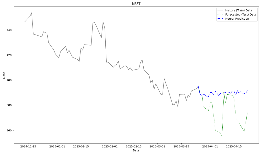
Not bad, huh? The model captured the general sideways trend, though it missed some fluctuations (because, well, the stock market is unpredictable! 📉📈).
🚀 Key Takeaways & Future Improvements
✅ What worked:
- LSTMs are great at learning stock trends.
- Scaling data and using dropout helped avoid overfitting.
🔧 What could be better:
- Add more features (news sentiment 🗞️, technical indicators 📊).
- Try bigger models (Transformer? GPT for stocks? 🤖).
💡 Final Thoughts
Predicting stocks with AI is challenging but exciting! While our LSTM did a decent job, the stock market is influenced by countless factors—politics, news, Elon Musk’s tweets 🐦—so perfect predictions are tough.
But hey, we’re one step closer to building a robo-investor! 🤖💰
What stock should we predict next? Let me know in the comments! 👇
Disclaimer: This is for educational purposes only. Don’t bet your life savings on AI predictions! 🚨
Happy trading! 🚀📊
Aboud