💡 How does Netflix know what you’ll binge-watch next? Or how do businesses predict future sales with impressive accuracy?
The magic behind these predictions is Regression—a fundamental technique in Machine Learning! 🚀
Whether it's forecasting house prices 🏡, stock trends 📈, or weather patterns 🌦️, regression plays a crucial role in making data-driven decisions. In this guide, we’ll break it all down—step by step—with easy explanations, real-world examples, and hands-on code.
🔍 What’s in store for you?
We'll explore various Regression algorithms, understand how they work, and see them in action with practical applications. Let’s dive in! 🔥
💡 1. Linear Regression: The Foundation of Predictive Modeling
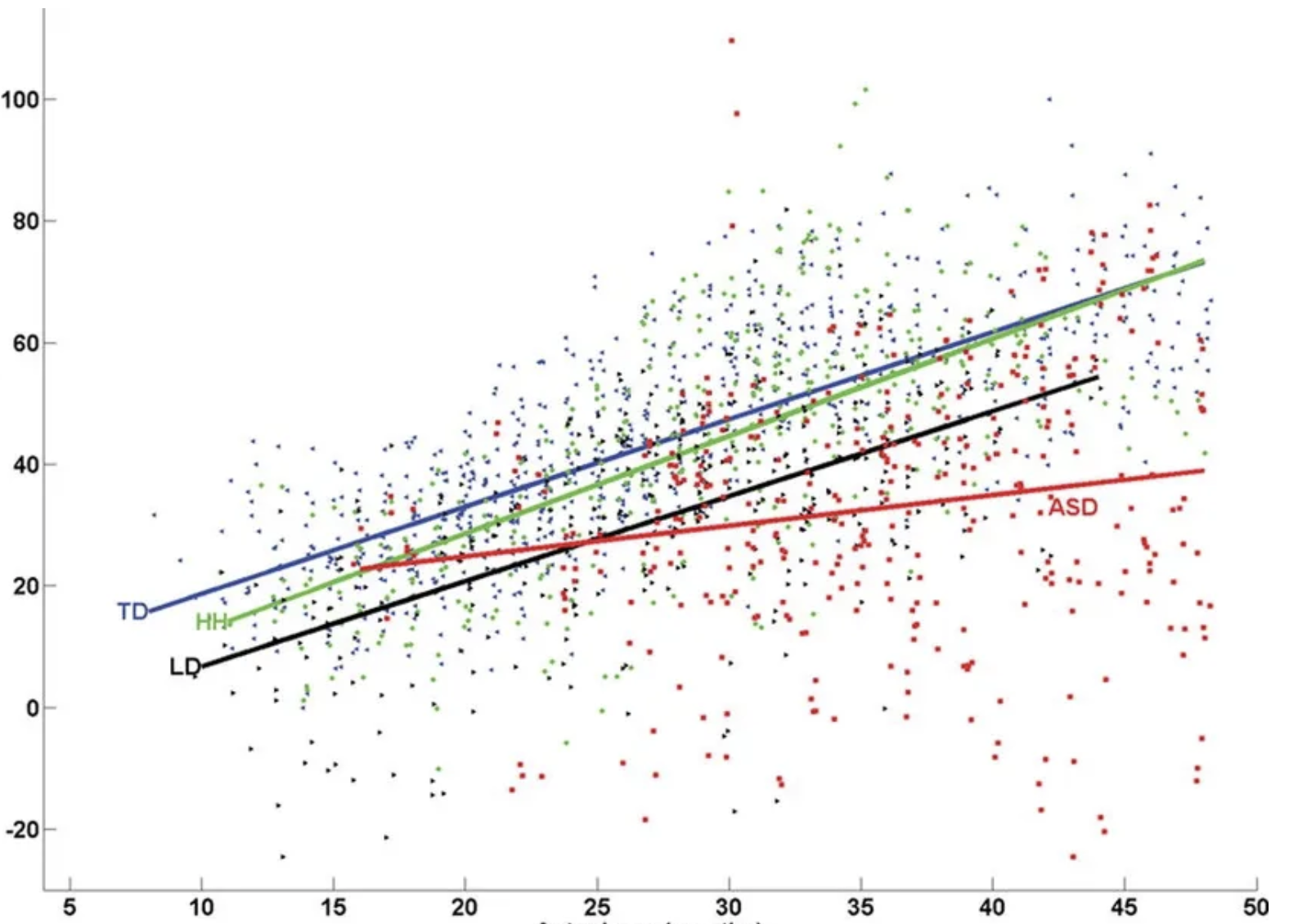
Linear Regression is the most fundamental regression technique, assuming a straight-line relationship between input variables (X) and the output (Y). It is widely used for predicting trends, making forecasts, and understanding relationships between variables.
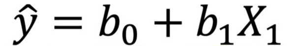
By fitting a linear equation to the observed data, Linear Regression helps in estimating the dependent variable based on independent variables. The equation of a simple linear regression is:
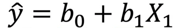
📌 Where:
- Y = Predicted value (dependent variable)
- X = Input feature (independent variable)
- b₀ = Intercept (constant term)
- b₁ = Slope (coefficient of X)
- ε = Error term
🔹 Key Applications of Linear Regression:
✅ Stock Market Predictions 📈
✅ Sales Forecasting 🛍️
✅ Real Estate Price Estimation 🏡
✅ Medical Research & Risk Analysis ⚕️
🖥️ Implementing Linear Regression in Python:
Let's implement Simple Linear Regression using Python and Scikit-Learn:
import numpy as np
import matplotlib.pyplot as plt
from sklearn.linear_model import LinearRegression
from sklearn.model_selection import train_test_split

# Sample dataset
data_X = np.array([1, 2, 3, 4, 5, 6, 7, 8, 9, 10]).reshape(-1, 1)
data_Y = np.array([3, 4, 2, 5, 6, 7, 8, 9, 10, 12])

# Splitting the data
X_train, X_test, Y_train, Y_test = train_test_split(data_X, data_Y, test_size=0.2, random_state=42)

# Model training
model = LinearRegression()
model.fit(X_train, Y_train)

# Predictions
y_pred = model.predict(X_test)

# Plotting the regression line
plt.scatter(data_X, data_Y, color='blue', label='Actual Data')
plt.plot(X_test, y_pred, color='red', linewidth=2, label='Regression Line')
plt.xlabel("Input Feature (X)")
plt.ylabel("Output (Y)")
plt.title("Linear Regression Model")
plt.legend()
plt.show()
📊 Output Visualization:
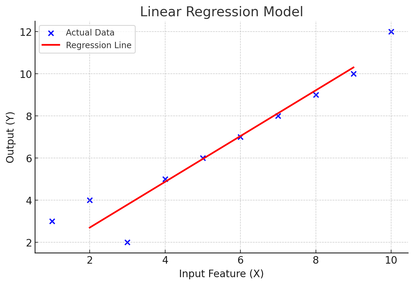
This simple example demonstrates how Linear Regression can be implemented using Scikit-Learn in Python. 🚀
Stay tuned as we explore more regression techniques in the next sections! 🔥
🔎 Example Use Case:
📌 Predicting house prices based on square footage 🏠
Imagine you have a dataset with house sizes and their respective prices. By applying Linear Regression, you can predict the price of a house based on its area!
📢 Tip: Always check model assumptions like linearity, independence, and normal distribution of residuals before applying Linear Regression in real-world scenarios.
Let’s move on to more advanced regression techniques in the next section! 🚀
🚀 2. Multiple Linear Regression: Expanding Predictive Power
Multiple Linear Regression extends Simple Linear Regression by incorporating multiple input variables to predict an outcome. Instead of modeling a relationship between just one independent variable and the dependent variable, it considers two or more independent variables, making predictions more accurate.
🔍 Understanding Multiple Linear Regression
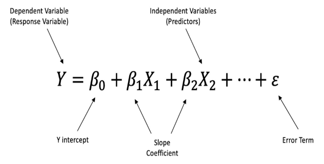
In Multiple Linear Regression, the relationship between the dependent variable (Y) and multiple independent variables (X₁, X₂, X₃, ... Xₙ) is represented as:
📏 Equation of Multiple Linear Regression:

Where:
- Y = Dependent variable (what we predict)
- X₁, X₂, X₃, ... Xₙ = Independent variables (input features)
- b₀ = Intercept (constant term)
- b₁, b₂, ..., bₙ = Coefficients representing the influence of each variable
- ε = Error term
📊 Visual Representation:
1️⃣ Concept of Multiple Regression
2️⃣ Regression Plane Representation (for 2 Variables)
3️⃣ Multiple Linear Regression Formula Breakdown
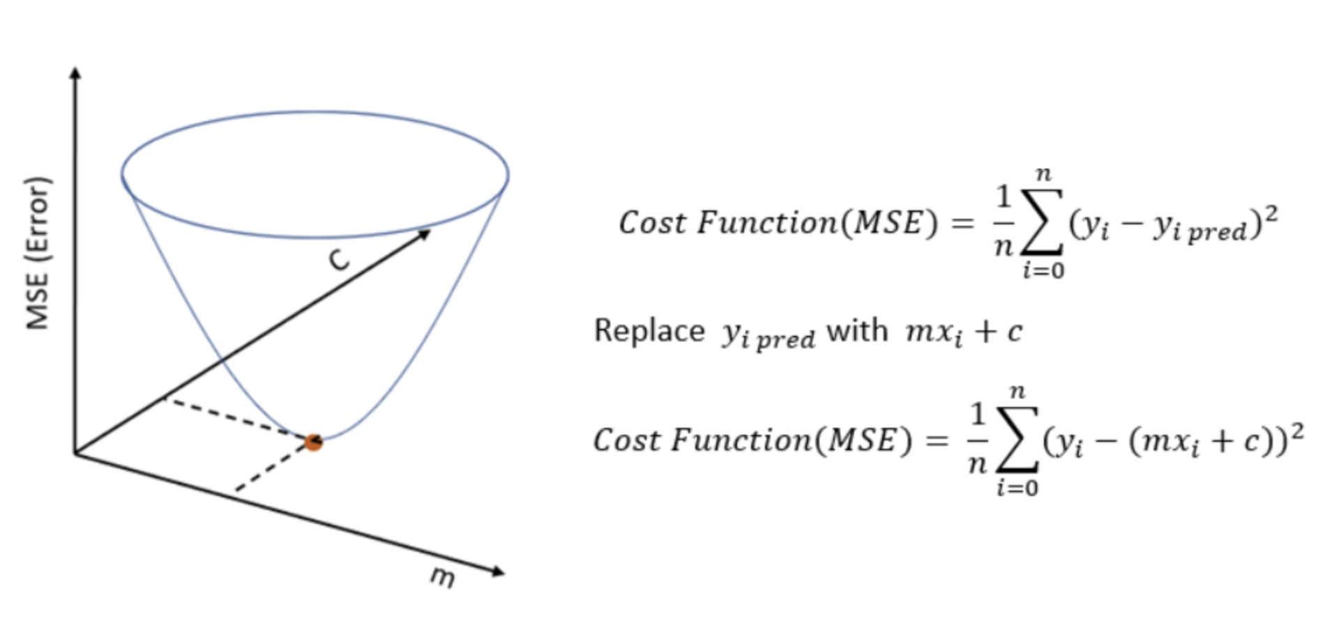
🖥️ Code Implementation: Mean Squared Error (MSE) in Python
import numpy as np

def mean_squared_error(y_actual, y_pred):
    """
    Compute the Mean Squared Error (MSE) cost function.

    Parameters:
    y_actual : np.array : Actual values
    y_pred : np.array : Predicted values (mx + c)

    Returns:
    float : MSE value
    """
    n = len(y_actual)  # Number of data points
    mse = (1 / n) * np.sum((y_actual - y_pred) ** 2)
    return mse

# Example Data
x = np.array([1, 2, 3, 4, 5])  # Input features
y_actual = np.array([2, 4, 6, 8, 10])  # Actual output values

# Linear regression parameters
m = 2  # Slope
c = 0  # Intercept

# Compute predictions
y_pred = m * x + c

# Compute MSE
mse_value = mean_squared_error(y_actual, y_pred)

print("Mean Squared Error (MSE):", mse_value)
🏠 Example Use Case: Predicting House Prices
Features considered:
- X₁: Size of the house (sq ft)
- X₂: Number of bedrooms
- X₃: Location rating
- Y: Predicted house price
✅ Advantages of Multiple Linear Regression:
✔️ Captures the effect of multiple variables for better predictions.
✔️ Useful for complex real-world scenarios like finance, healthcare, and business analytics.
❌ Challenges of Multiple Linear Regression:
⚠️ More features increase complexity and overfitting risks.
⚠️ Requires careful feature selection and normalization for accuracy.
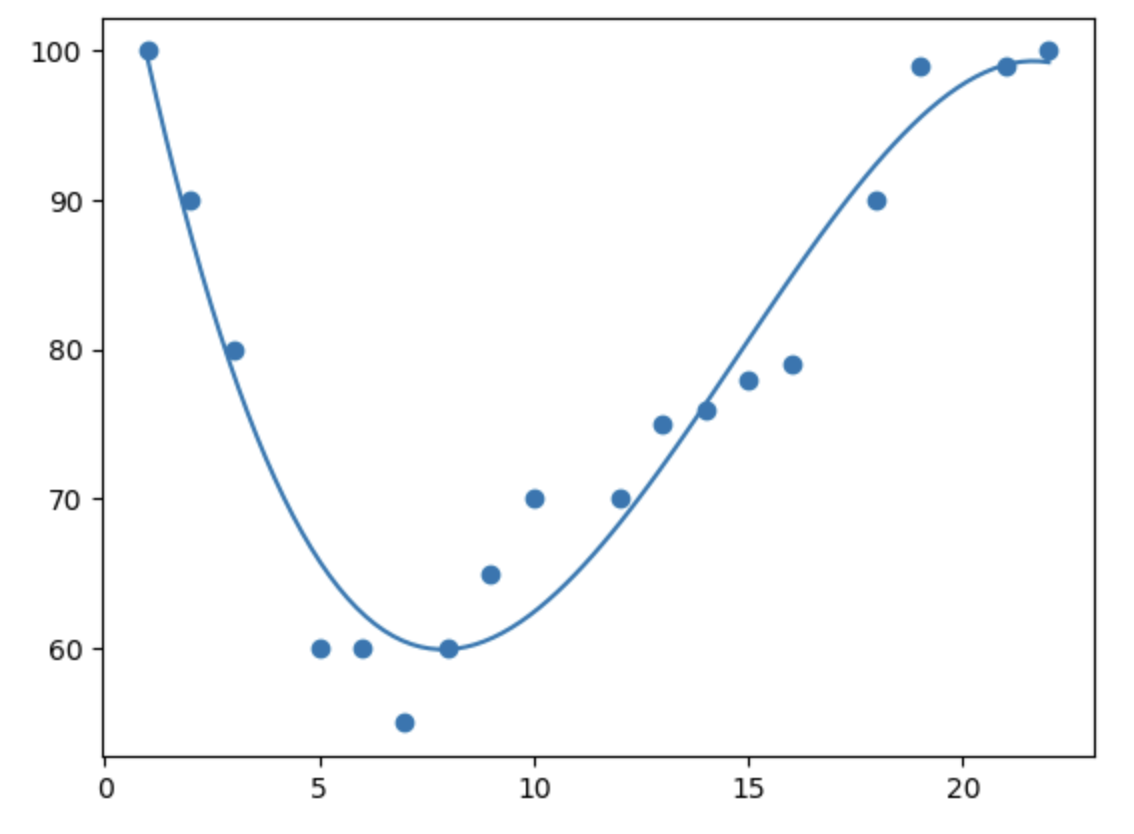
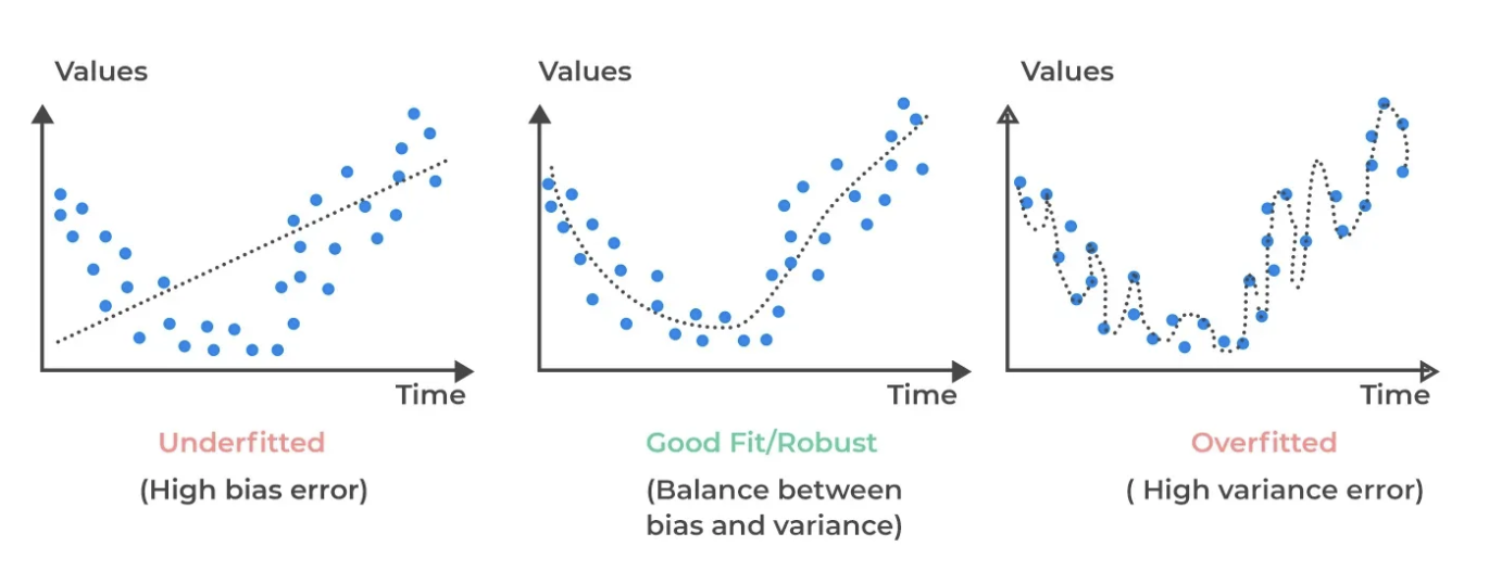
🚀 3. Polynomial Regression: Capturing Non-Linear Trends
When data doesn’t follow a straight-line trend, Polynomial Regression helps model non-linear relationships by introducing polynomial terms to the equation. This technique is useful when the relationship between the independent and dependent variables is curved.
📌 Equation:
Polynomial Regression extends Linear Regression by incorporating higher-degree polynomial terms:
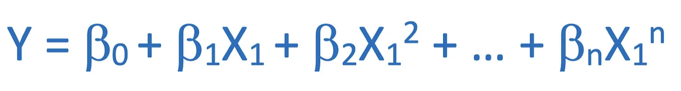
Where:
- Y is the predicted output
- X is the input feature
- b₀, b₁, b₂, …, bₙ are the regression coefficients
- n is the polynomial degree
- ε is the error term
🔍 Real-World Applications of Polynomial Regression:
- 📈 Salary Prediction: Estimating salary growth over time, where experience influences salary in a non-linear fashion.
- 🦠 COVID-19 Trend Forecasting: Modeling infection rate trends, which often follow polynomial or exponential growth.
- 🚗 Vehicle Performance Modeling: Predicting fuel consumption based on speed and engine performance.
- 📊 Economics & Finance: Forecasting demand, inflation, and economic trends where relationships are complex.
✅ Advantages:
✔️ Works well for curved datasets where Linear Regression fails.
✔️ Provides a better fit for non-linear trends when the correct degree is chosen.
❌ Disadvantages:
❌ Can overfit the data if the polynomial degree is too high.
❌ Harder to interpret compared to simple Linear Regression.
🖥️ Python Code for Polynomial Regression:
import numpy as np
import matplotlib.pyplot as plt
from sklearn.preprocessing import PolynomialFeatures
from sklearn.linear_model import LinearRegression
from sklearn.pipeline import make_pipeline

# Sample dataset
X = np.array([1, 2, 3, 4, 5, 6, 7, 8, 9, 10]).reshape(-1, 1)
y = np.array([2, 5, 10, 18, 30, 50, 75, 105, 140, 180])

# Creating a polynomial model (degree = 2)
poly_model = make_pipeline(PolynomialFeatures(degree=2), LinearRegression())
poly_model.fit(X, y)

y_pred = poly_model.predict(X)

# Plot results
plt.scatter(X, y, color='blue', label='Actual Data')
plt.plot(X, y_pred, color='red', linewidth=2, label='Polynomial Regression Line')
plt.xlabel("Input Feature (X)")
plt.ylabel("Output (Y)")
plt.title("Polynomial Regression Model")
plt.legend()
plt.show()
📌 Visual Representation:
Polynomial Regression allows machine learning models to capture non-linear relationships and make better predictions in real-world scenarios. 🚀
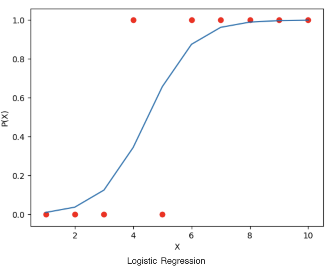
4. Logistic Regression (For Classification) :
Although it contains "Regression" in its name, Logistic Regression is used for Classification problems, not Regression.
Instead of predicting continuous values, it predicts probabilities and assigns categories like Yes/No, Pass/Fail, Spam/Not Spam.
Equation:
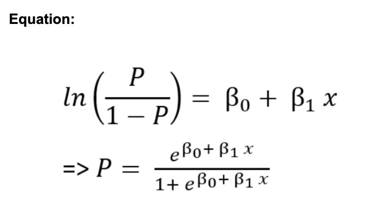
where P is the probability of belonging to a class.
✅ Example:
- Predicting whether a customer will buy a product (Yes/No).
- Classifying emails as spam or not.
✅ Why is it called Regression?
Although it’s used for classification, Logistic Regression applies a regression-based approach before applying the Sigmoid function to convert outputs into probabilities.
🖥️ Python Implementation of Logistic Regression
import numpy as np
import matplotlib.pyplot as plt
from sklearn.model_selection import train_test_split
from sklearn.linear_model import LogisticRegression
from sklearn.metrics import accuracy_score, classification_report

# Sample dataset (Binary classification: Pass (1) or Fail (0))
X = np.array([[20], [25], [30], [35], [40], [45], [50], [55], [60], [65]])  # Hours studied
y = np.array([0, 0, 0, 1, 1, 1, 1, 1, 1, 1])  # 0 = Fail, 1 = Pass

# Splitting dataset
X_train, X_test, y_train, y_test = train_test_split(X, y, test_size=0.2, random_state=42)

# Training Logistic Regression model
model = LogisticRegression()
model.fit(X_train, y_train)

# Predictions
y_pred = model.predict(X_test)

# Evaluating model
accuracy = accuracy_score(y_test, y_pred)
print("Accuracy:", accuracy)
print("Classification Report:\n", classification_report(y_test, y_pred))

# Plotting the sigmoid curve
X_range = np.linspace(15, 70, 100).reshape(-1, 1)
y_probs = model.predict_proba(X_range)[:, 1]

plt.scatter(X, y, color='blue', label='Actual Data')
plt.plot(X_range, y_probs, color='red', label='Sigmoid Curve')
plt.xlabel("Hours Studied")
plt.ylabel("Probability of Passing")
plt.title("Logistic Regression Model")
plt.legend()
plt.show()
📌 Expected Output:
Accuracy: 1.0  # (Might vary slightly depending on random split)
Classification Report:
              precision    recall  f1-score   support

           0       1.00      1.00      1.00         1
           1       1.00      1.00      1.00         1

    accuracy                           1.00         2
   macro avg       1.00      1.00      1.00         2
weighted avg       1.00      1.00      1.00         2
This implementation demonstrates how Logistic Regression is used for binary classification. The model predicts whether a student will pass or fail based on study hours, and we visualize the sigmoid function curve. 📊🔥
📌 Conclusion: Regression in Machine Learning
Regression is a fundamental concept in Machine Learning, enabling us to make continuous predictions based on input features. It is widely used in forecasting, trend analysis, and data-driven decision-making.
🔹 Quick Summary of Regression Algorithms
| Algorithm | Use Case | Equation Type | Best For |
|---|---|---|---|
| Linear Regression | Predicting sales, stock prices | Linear equation | Simple relationships between variables |
| Multiple Regression | House pricing with multiple factors | Linear (Multiple Inputs) | Impact of multiple features |
| Polynomial Regression | Salary growth trends, COVID-19 cases | Polynomial equation | Capturing non-linear patterns |
| Logistic Regression | Spam detection, customer conversion | Sigmoid function | Classification problems |
🏆 Key Takeaways
✅ Regression is essential for predictive modeling in real-world applications.
✅ Choosing the right regression technique depends on data patterns and relationships.
✅ Logistic Regression is used for classification, despite its name.
Regression models power AI-driven decision-making, forming the backbone of modern analytics and forecasting! 🚀